16: Conditioning the Landscape (Batch Norm)

The Landscape Geometry Problem

So far, we have discussed “Sharp vs Flat” minima. But there is another geometric feature that ruins SGD’s day: Eccentricity.

Ideally, we want our loss function to look like a perfect bowl (Circle).

• Gradient points directly to the center.
• We can take a straight path to the minimum.

In reality, most loss functions are elongated valleys (Ellipses).

• Steep in one direction (Walls of the valley).
• Flat in the other direction (Floor of the valley).

The “Bouncing” Problem

Because the gradient corresponds to steepness, it is massive in the “steep” direction and tiny in the “flat” direction.

• SGD takes a huge step into the wall, overshoots, and bounces back.
• It barely moves along the valley floor. This zig-zagging behavior makes convergence painfully slow.

---

1. Visualizing Ill-Conditioning

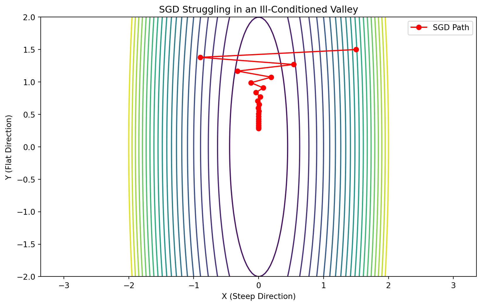
Let’s visualize SGD trying to optimize a skewed quadratic bowl: f(x,y) = 10x^2 + y^2. * This valley is 10x steeper in x than y. * The Condition Number (Ratio of curvature) is 10.

Code

import numpy as np
import matplotlib.pyplot as plt

def skewed_loss(x, y):
    return 20*x**2 + y**2  # Very steep in X, flat in Y

def skewed_grad(x, y):
    return np.array([40*x, 2*y])

# Run SGD
lr = 0.04 # If we set this for the flat direction (y), x will explode!
w = np.array([1.5, 1.5])
path_x, path_y = [w[0]], [w[1]]

for _ in range(20):
    g = skewed_grad(w[0], w[1])
    w = w - lr * g
    path_x.append(w[0])
    path_y.append(w[1])

# Plot
x_grid = np.linspace(-2, 2, 100)
y_grid = np.linspace(-2, 2, 100)
X, Y = np.meshgrid(x_grid, y_grid)
Z = skewed_loss(X, Y)

plt.figure(figsize=(10, 6))
plt.contour(X, Y, Z, levels=20, cmap='viridis')
plt.plot(path_x, path_y, 'r-o', label="SGD Path")
plt.title("SGD Struggling in an Ill-Conditioned Valley")
plt.xlabel("X (Steep Direction)")
plt.ylabel("Y (Flat Direction)")
plt.legend()
plt.axis('equal')
plt.show()

Notice the zig-zag. The optimizer is fighting the geometry. To stop the bouncing in x, we’d have to lower the Learning Rate. But if we lower the LR, progress in y becomes glacial.

---

2. Feature Scaling: The First Fix

The simplest fix is one you learn in any introductory Machine Learning course: Standardize your data.

If we scale the inputs so they have unit variance (x' = x / \sigma), we essentially squash the ellipse into a circle.

Mathematically, this improves the Condition Number of the Hessian matrix. Consider a linear regression problem y = Xw. The Hessian is H = X^T X. The closer X is to orthogonal (spherical), the closer H is to the identity matrix, and the faster Gradient Descent converges.

But here is the catch: Standardizing the input dataset (X) only fixes the condition number for the first layer of weights. What about the rest of the network?

---

3. Batch Norm: Dynamic Conditioning

In a deep model (or any chained optimization problem), the “inputs” to Layer 2 are the “outputs” of Layer 1. h_1 = \sigma(W_1 x) h_2 = \sigma(W_2 h_1)

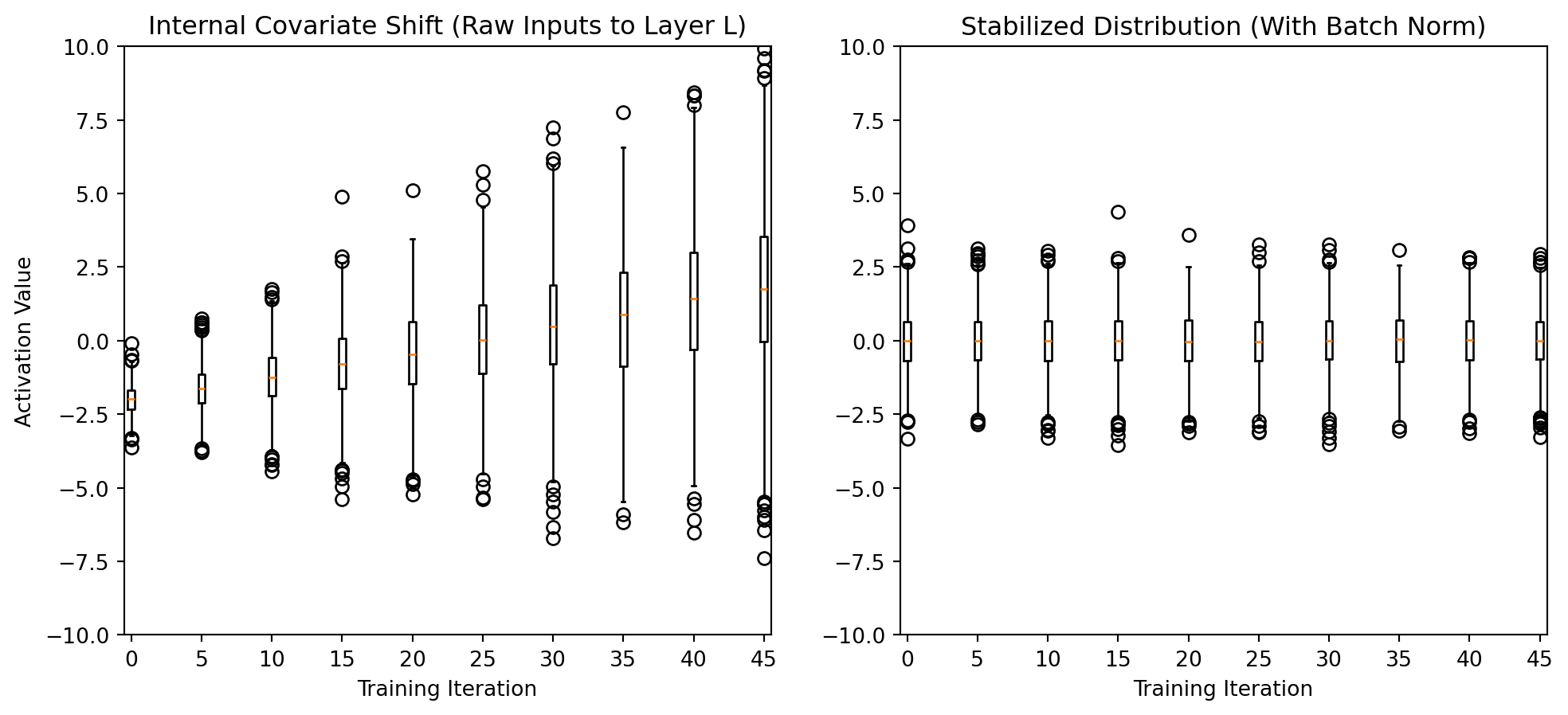
As the optimizer updates W_1, the distribution of h_1 shifts wildly. This means Layer 2 is constantly trying to chase a moving target. Its “input features” are changing scale and shape every iteration. This is called Internal Covariate Shift.

Batch Normalization (BN) is simply the idea of applying that “Standardization Fix” continuously throughout the optimization graph.

The Mechanism

Before passing the data to the next layer, we force it to be spherical. For every mini-batch B: \mu_B = \text{mean}(h_1) \quad \sigma_B^2 = \text{variance}(h_1) \hat{h}_1 = \frac{h_1 - \mu_B}{\sqrt{\sigma_B^2 + \epsilon}}

How it changes Optimization Geometry

It is not just about “better features”. It is a geometric transformation of the optimization landscape itself.

By forcing every intermediate signal to have mean 0 and variance 1:

1. Sphering: We force the “Ellipses” to stay “Circular” locally at every layer.
2. Length Independence: Scaling the weights by a constant factor (2W) effectively cancels out because the normalization divides by that same factor. This removes the “scale” degree of freedom, simplifying the search space.
3. Stability: We can use massive Learning Rates without bouncing off the walls, because the landscape no longer has “sharp, steep walls” caused by exploding signal variance.

Code

# Simple Visualization of Covariate Shift vs Batch Norm
# We generate random data that drifts over time (Shift)
# And show how BN keeps it stable.

np.random.seed(42)
steps = 50
means = np.linspace(-2, 2, steps)
stds = np.linspace(0.5, 3.0, steps)

raw_data = []
bn_data = []

for m, s in zip(means, stds):
    # Simulate the "Shift": Distribution changes every step
    batch = np.random.normal(m, s, 1000)
    raw_data.append(batch)
    
    # Apply Batch Norm Fix
    bn_batch = (batch - np.mean(batch)) / np.std(batch)
    bn_data.append(bn_batch)

# Plotting the Distributions over time (Boxplots)
fig, (ax1, ax2) = plt.subplots(1, 2, figsize=(12, 5))

ax1.boxplot(raw_data[::5], positions=np.arange(0, 50, 5))
ax1.set_title("Internal Covariate Shift (Raw Inputs to Layer L)")
ax1.set_xlabel("Training Iteration")
ax1.set_ylabel("Activation Value")
ax1.set_ylim(-10, 10)

ax2.boxplot(bn_data[::5], positions=np.arange(0, 50, 5))
ax2.set_title("Stabilized Distribution (With Batch Norm)")
ax2.set_xlabel("Training Iteration")
ax2.set_ylim(-10, 10) # Same scale

plt.show()

• Left (Raw): The inputs to the layer are drifting (mean moves up) and exploding (variance grows). The weights W_L have to constantly re-adapt to this changing scale.

• Right (BN): The inputs are locked. They always look like a standard Gaussian. The weights W_L can focus purely on learning the pattern rather than chasing the scale.

---

4. Simulation: Conditioning the Landscape

Let’s simulate a deep linear chain (5 matrix multiplications) to optimize y = W_5 W_4 W_3 W_2 W_1 x.

This is a convex problem (it collapses to a single linear layer), but it is extremely ill-conditioned to train layer-by-layer. Only specific directions in the parameter space preserve the signal magnitude, while others kill it.

We will compare:

1. Standard SGD: Standard chain.
2. SGD + BatchNorm: We normalize the signal after every multiplication.

Code

# Simulation of Deep Linear Network signal propagation
# We track the loss convergence to see if it vanishes/explodes

dims = 50
depth = 10
batch_size = 32

np.random.seed(42)

# Input Data & Target
X = np.random.randn(batch_size, dims)
y_target = np.random.randn(batch_size, dims) # Dummy target

# Initialize Weights (Same seeds)
weights_std = [np.random.randn(dims, dims) * 0.1 for _ in range(depth)]
weights_bn = [w.copy() for w in weights_std] # Exact same start

# SGD Settings
lr = 0.05 
losses_std = []
losses_bn = []

# Training Loop
for step in range(200):
    
    # --- A. Standard Net Forward ---
    h = X.copy()
    cache_std = [h]
    for W in weights_std:
        h = h @ W
        cache_std.append(h)
    
    loss_std = np.mean((h - y_target)**2)
    losses_std.append(loss_std)
    
    # Standard Backward (Chain Rule)
    grad_h = 2 * (h - y_target) / batch_size
    for i in reversed(range(depth)):
        W = weights_std[i]
        h_prev = cache_std[i]
        
        dW = h_prev.T @ grad_h
        grad_h = grad_h @ W.T # Pass grad back
        
        weights_std[i] -= lr * dW
        
    # --- B. BN Net Forward ---
    # Concept: h = Norm(h @ W)
    h_bn = X.copy()
    cache_bn = [h_bn]
    for i, W in enumerate(weights_bn):
        z = h_bn @ W
        
        # Batch Norm Logic applied manually
        mean = np.mean(z, axis=0)
        std = np.std(z, axis=0) + 1e-8
        h_bn = (z - mean) / std # Normalize!
        
        cache_bn.append(h_bn)
        
    loss_bn = np.mean((h_bn - y_target)**2)
    losses_bn.append(loss_bn)
    
    # BN Backward (Approximate for demonstration)
    # We essentially update weights using the "Normalized" signal gradient.
    # This captures the main benefit: the GRADIENT scale is stabilized.
    grad_h_bn = 2 * (h_bn - y_target) / batch_size
    for i in reversed(range(depth)):
        W = weights_bn[i]
        h_prev = cache_bn[i]
        
        dW = h_prev.T @ grad_h_bn
        grad_h_bn = grad_h_bn @ W.T
        
        weights_bn[i] -= lr * dW # Same LR!

plt.figure(figsize=(10, 6))
plt.plot(losses_std, label="Standard Chains (Ill-Conditioned)", linestyle='--', color='blue')
plt.plot(losses_bn, label="Conditioned Chains (Batch Norm)", linewidth=2, color='orange')

plt.title("Optimizing a Deep Linear Chain ($W_{10}...W_1 x$)")
plt.xlabel("Iteration")
plt.ylabel("MSE Loss (Log Scale)")
plt.legend()
plt.yscale('log')
plt.grid(True, alpha=0.3)
plt.show()

/home/kmcalist/.local/lib/python3.10/site-packages/numpy/core/_methods.py:176: RuntimeWarning:

overflow encountered in multiply

/tmp/ipykernel_2571803/3313781696.py:73: RuntimeWarning:

overflow encountered in matmul

/tmp/ipykernel_2571803/3313781696.py:30: RuntimeWarning:

overflow encountered in matmul

/tmp/ipykernel_2571803/3313781696.py:30: RuntimeWarning:

invalid value encountered in matmul

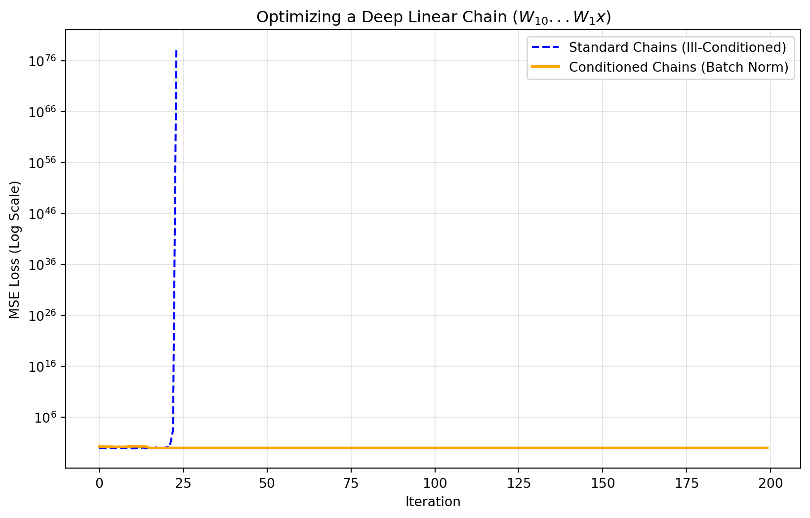
• The Standard Optimization (Blue) struggles. The chain of multiplications creates an ill-conditioned landscape where gradients are extremely sensitive. It gets stuck at a high loss.

• The Conditioned Optimization (Orange) drops like a rock. By keeping the signal “spherical” (normalized) at every step, we effectively precondition the problem, making SGD incredibly efficient even through 10 layers.

For modern problems that have a long chain of gradients that are multiplied to compute downstream gradients, batch norm isn’t just a suggestion - it’s a necessity.