(Note: Adam also includes a “bias correction” step to prevent cold starts, ensuring m_t and v_t don’t stick to zero at the very beginning).
How Does it Perform?
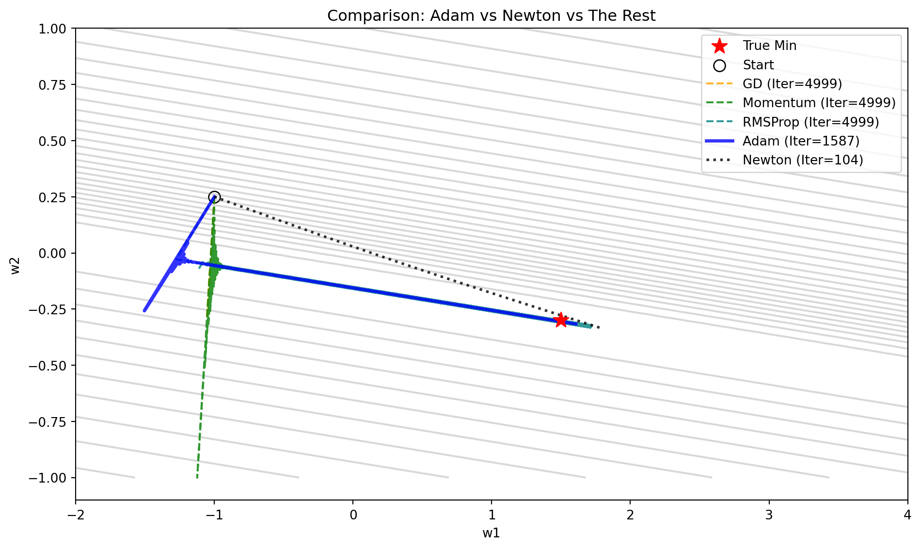
Let’s run the final competition on our “Narrow Valley”. We will pit the four major algorithms against each other:
Gradient Descent (Baseline)
Momentum (Fast but needs scaling)
RMSProp (Scales well but zig-zags)
Adam (The Combine)
Newton (The Gold Standard)
Code
import numpy as npimport matplotlib.pyplot as pltimport timefrom IPython.display import Markdown# -----------------------------# 1. Setup the Nasty Valley (Same as before)# -----------------------------np.random.seed(42)n =10_000x1 = np.random.normal(0, 1, n)x2 =10.0* x1 + np.random.normal(0, .5, n) X = np.column_stack([x1, x2])w_true = np.array([1.5, -0.3]) logits = X @ w_truep =1/ (1+ np.exp(-logits))y = np.random.binomial(1, p)def get_loss(w): p =1/ (1+ np.exp(-X @ w)) eps =1e-12return-np.average(y * np.log(p + eps) + (1- y) * np.log(1- p + eps))def get_grad(w): p =1/ (1+ np.exp(-X @ w))return (X.T @ (p - y)) / ndef get_hessian(w): p =1/ (1+ np.exp(-X @ w)) weights = p * (1- p)return (X.T @ (weights[:, None] * X)) / n# -----------------------------# 2. Run Algorithms# -----------------------------w_start = np.array([-1.0, 0.25])tol =1e-4max_iter =5000results = []# --- A. Gradient Descent ---w = w_start.copy()path_gd = [w.copy()]start = time.time()converged =Falsefor i inrange(max_iter): grad = get_grad(w)if np.linalg.norm(grad) < tol: converged =True;break w = w -0.1* grad path_gd.append(w.copy())results.append({"name": "GD", "path": np.array(path_gd), "time": time.time()-start, "iters": i, "conv": converged})# --- B. Momentum ---w = w_start.copy()v = np.zeros_like(w)path_mom = [w.copy()]start = time.time()converged =Falsebeta =0.9for i inrange(max_iter): grad = get_grad(w)if np.linalg.norm(grad) < tol: converged =True;break v = beta * v +0.1* grad w = w - v path_mom.append(w.copy())results.append({"name": "Momentum", "path": np.array(path_mom), "time": time.time()-start, "iters": i, "conv": converged})# --- C. RMSProp ---w = w_start.copy()r = np.zeros_like(w)path_rms = [w.copy()]start = time.time()converged =Falseeta =0.01beta =0.9for i inrange(max_iter): grad = get_grad(w)if np.linalg.norm(grad) < tol: converged =True;break r = beta * r + (1- beta) * grad**2 w = w - (eta / (np.sqrt(r) +1e-8)) * grad path_rms.append(w.copy())results.append({"name": "RMSProp", "path": np.array(path_rms), "time": time.time()-start, "iters": i, "conv": converged})# --- D. Adam ---w = w_start.copy()m = np.zeros_like(w)v = np.zeros_like(w)path_adam = [w.copy()]start = time.time()converged =Falseeta =0.1beta1 =0.9beta2 =0.999for i inrange(max_iter): t = i +1 grad = get_grad(w)if np.linalg.norm(grad) < tol: converged =True;break# 1. Update Momentum m = beta1 * m + (1- beta1) * grad# 2. Update Velocity v = beta2 * v + (1- beta2) * grad**2# 3. Bias Correction m_hat = m / (1- beta1**t) v_hat = v / (1- beta2**t) w = w - eta * m_hat / (np.sqrt(v_hat) +1e-8) path_adam.append(w.copy())results.append({"name": "Adam", "path": np.array(path_adam), "time": time.time()-start, "iters": i, "conv": converged})# --- E. Newton's Method (The Gold Standard) ---w = w_start.copy()path_newt = [w.copy()]start = time.time()converged =Falsefor i inrange(max_iter): grad = get_grad(w)if np.linalg.norm(grad) < tol: converged =True;break H = get_hessian(w)try: step = np.linalg.solve(H, grad)except np.linalg.LinAlgError:break w = w -0.1* step # Small step for stability path_newt.append(w.copy())results.append({"name": "Newton", "path": np.array(path_newt), "time": time.time()-start, "iters": i, "conv": converged})# -----------------------------# 3. Visualization# -----------------------------w1_vals = np.linspace(-2, 4, 100)w2_vals = np.linspace(-1, 1, 100)W1, W2 = np.meshgrid(w1_vals, w2_vals)Z = np.zeros_like(W1)for i inrange(W1.shape[0]):for j inrange(W1.shape[1]): Z[i,j] = get_loss(np.array([W1[i,j], W2[i,j]]))plt.figure(figsize=(10, 6))plt.contour(W1, W2, Z, levels=np.logspace(np.log10(Z.min()), np.log10(Z.max()), 30), colors='gray', alpha=0.3)plt.scatter(w_true[0], w_true[1], c='red', marker='*', s=150, zorder=10, label="True Min")plt.scatter(w_start[0], w_start[1], c='white', edgecolors='black', s=80, label="Start")colors = ['orange', 'green', 'teal', 'blue', 'black']styles = ['--', '--', '--', '-', ':']widths = [1.5, 1.5, 1.5, 2.5, 2.0]for idx, res inenumerate(results): path = res['path'] plt.plot(path[:,0], path[:,1], styles[idx], label=f"{res['name']} (Iter={res['iters']})", color=colors[idx], markersize=3, alpha=0.8, linewidth=widths[idx])plt.title("Comparison: Adam vs Newton vs The Rest")plt.xlabel("w1")plt.ylabel("w2")plt.legend()plt.tight_layout()plt.show()# -----------------------------# 4. Results Table# -----------------------------table_md ="""| Algorithm | Iterations | Total Time (s) | Time/Iter (ms) | Final w | Status ||---|---|---|---|---|---|"""for res in results: s ="Converged ✅"if res['conv'] else"Slow ⏳" w_s =f"({res['path'][-1][0]:.3f}, {res['path'][-1][1]:.3f})" t_per = (res['time'] / res['iters']) *1000if res['iters'] >0else0 table_md +=f"| {res['name']} | {res['iters']} | {res['time']:.4f} | {t_per:.3f} | {w_s} | {s} |\n"Markdown(table_md)
Algorithm
Iterations
Total Time (s)
Time/Iter (ms)
Final w
Status
GD
4999
0.2196
0.044
(-0.485, -0.107)
Slow ⏳
Momentum
4999
0.3790
0.076
(1.459, -0.301)
Slow ⏳
RMSProp
4999
0.2597
0.052
(1.723, -0.323)
Slow ⏳
Adam
1587
0.0907
0.057
(1.607, -0.316)
Converged ✅
Newton
104
0.0139
0.134
(1.786, -0.334)
Converged ✅
Adam combines the best of both first order improvements and converges quicker than the rest. It is slower than Newton in this simple problem, but the inversion of the Hessian will quickly become unruly and Adam will be the winner.
Practical Implementation
In practice, you rarely implement Adam from scratch. Modern frameworks like PyTorch and TensorFlow provide highly optimized implementations.
Standard Hyperparameters
Unlike Gradient Descent or Momentum where you often have to tune multiple knobs, Adam is famous for working well “out of the box” with standard defaults.
Learning Rate (\alpha): Usually 0.001 or 3e-4 (often called “Karpathy’s Constant”).
\beta_1 (Momentum): 0.9
\beta_2 (Scaling): 0.999
\epsilon: 1e-8 (for numerical stability)
While Adam is less sensitive to the Learning Rate than GD, it is not immune (as we saw with Momentum). You usually don’t need to grid search nearly as extensively, but it is still standard practice to try logarithmic steps (e.g., 1e-2, 1e-3, 1e-4) to find the right magnitude using a LR search. It is also good practice to pair Adam with a learning rate decay scheduler.
Is extensive tuning necessary? Generally, no. Unlike GD, where the optimal learning rate can vary wildly between problems, Adam usually works within a consistent order of magnitude.
Run a simple Learning Rate Finder (fast scan for 1 epoch) to identify the maximum stable learning rate.
Set your LR slightly below that peak (e.g., divide by 10).
Let the adaptive nature of Adam handle the rest.
Unless you are training a state-of-the-art model where every 0.1% accuracy counts, you rarely need to run expensive multi-epoch grid searches for Adam’s learning rate.
The AdamW Variant
If you are doing anything related to Transformers (BERT, GPT, Attention), you should use AdamW instead of standard Adam.
The original Adam paper had a small inconsistency in how it handled Weight Decay (L2 Regularization).
Adam: Incorporates weight decay into the gradient. This means the regularization gets scaled by the adaptive term v_t, effectively shrinking the regularization strength when gradients are large.
AdamW: Decouples weight decay, applying it directly to the weights after the main update. This ensures consistent regularization regardless of how the gradient is scaled.
For simple problems, they behave similarly. For state-of-the-art Deep Learning, AdamW generalizes significantly better.
Source Code
---title: "11: The Modern Optimizer: Adam"format: html: code-fold: truejupyter: python3---## The Best of Both WorldsWe have seen two powerful distinct ideas:1. **Momentum** (Tab 09): Accumulates a history of gradients to smooth out the zig-zags. This acts like the **Rotation** aspect of Newton's method.2. **RMSProp** (Tab 10): Accumulates a history of *squared* gradients to scale the step sizes. This acts like the **Scaling** aspect of Newton's method.It was only a matter of time before someone combined them.**Adam (Adaptive Moment Estimation)**, proposed by Kingma & Ba (2014), does exactly this. It maintains two separate history buffers:1. $m_t$: Exponential moving average of gradients (Momentum).2. $v_t$: Exponential moving average of squared gradients (RMSProp).$$\begin{align}m_t &= \beta_1 m_{t-1} + (1-\beta_1) \nabla L \\v_t &= \beta_2 v_{t-1} + (1-\beta_2) (\nabla L)^2\end{align}$$It then computes the update using both:$$ w_{t+1} = w_t - \eta \frac{m_t}{\sqrt{v_t} + \epsilon} $$*(Note: Adam also includes a "bias correction" step to prevent cold starts, ensuring $m_t$ and $v_t$ don't stick to zero at the very beginning).*---## How Does it Perform?Let's run the final competition on our "Narrow Valley". We will pit the four major algorithms against each other:1. **Gradient Descent** (Baseline)2. **Momentum** (Fast but needs scaling)3. **RMSProp** (Scales well but zig-zags)4. **Adam** (The Combine)5. **Newton** (The Gold Standard)```{python}import numpy as npimport matplotlib.pyplot as pltimport timefrom IPython.display import Markdown# -----------------------------# 1. Setup the Nasty Valley (Same as before)# -----------------------------np.random.seed(42)n =10_000x1 = np.random.normal(0, 1, n)x2 =10.0* x1 + np.random.normal(0, .5, n) X = np.column_stack([x1, x2])w_true = np.array([1.5, -0.3]) logits = X @ w_truep =1/ (1+ np.exp(-logits))y = np.random.binomial(1, p)def get_loss(w): p =1/ (1+ np.exp(-X @ w)) eps =1e-12return-np.average(y * np.log(p + eps) + (1- y) * np.log(1- p + eps))def get_grad(w): p =1/ (1+ np.exp(-X @ w))return (X.T @ (p - y)) / ndef get_hessian(w): p =1/ (1+ np.exp(-X @ w)) weights = p * (1- p)return (X.T @ (weights[:, None] * X)) / n# -----------------------------# 2. Run Algorithms# -----------------------------w_start = np.array([-1.0, 0.25])tol =1e-4max_iter =5000results = []# --- A. Gradient Descent ---w = w_start.copy()path_gd = [w.copy()]start = time.time()converged =Falsefor i inrange(max_iter): grad = get_grad(w)if np.linalg.norm(grad) < tol: converged =True;break w = w -0.1* grad path_gd.append(w.copy())results.append({"name": "GD", "path": np.array(path_gd), "time": time.time()-start, "iters": i, "conv": converged})# --- B. Momentum ---w = w_start.copy()v = np.zeros_like(w)path_mom = [w.copy()]start = time.time()converged =Falsebeta =0.9for i inrange(max_iter): grad = get_grad(w)if np.linalg.norm(grad) < tol: converged =True;break v = beta * v +0.1* grad w = w - v path_mom.append(w.copy())results.append({"name": "Momentum", "path": np.array(path_mom), "time": time.time()-start, "iters": i, "conv": converged})# --- C. RMSProp ---w = w_start.copy()r = np.zeros_like(w)path_rms = [w.copy()]start = time.time()converged =Falseeta =0.01beta =0.9for i inrange(max_iter): grad = get_grad(w)if np.linalg.norm(grad) < tol: converged =True;break r = beta * r + (1- beta) * grad**2 w = w - (eta / (np.sqrt(r) +1e-8)) * grad path_rms.append(w.copy())results.append({"name": "RMSProp", "path": np.array(path_rms), "time": time.time()-start, "iters": i, "conv": converged})# --- D. Adam ---w = w_start.copy()m = np.zeros_like(w)v = np.zeros_like(w)path_adam = [w.copy()]start = time.time()converged =Falseeta =0.1beta1 =0.9beta2 =0.999for i inrange(max_iter): t = i +1 grad = get_grad(w)if np.linalg.norm(grad) < tol: converged =True;break# 1. Update Momentum m = beta1 * m + (1- beta1) * grad# 2. Update Velocity v = beta2 * v + (1- beta2) * grad**2# 3. Bias Correction m_hat = m / (1- beta1**t) v_hat = v / (1- beta2**t) w = w - eta * m_hat / (np.sqrt(v_hat) +1e-8) path_adam.append(w.copy())results.append({"name": "Adam", "path": np.array(path_adam), "time": time.time()-start, "iters": i, "conv": converged})# --- E. Newton's Method (The Gold Standard) ---w = w_start.copy()path_newt = [w.copy()]start = time.time()converged =Falsefor i inrange(max_iter): grad = get_grad(w)if np.linalg.norm(grad) < tol: converged =True;break H = get_hessian(w)try: step = np.linalg.solve(H, grad)except np.linalg.LinAlgError:break w = w -0.1* step # Small step for stability path_newt.append(w.copy())results.append({"name": "Newton", "path": np.array(path_newt), "time": time.time()-start, "iters": i, "conv": converged})# -----------------------------# 3. Visualization# -----------------------------w1_vals = np.linspace(-2, 4, 100)w2_vals = np.linspace(-1, 1, 100)W1, W2 = np.meshgrid(w1_vals, w2_vals)Z = np.zeros_like(W1)for i inrange(W1.shape[0]):for j inrange(W1.shape[1]): Z[i,j] = get_loss(np.array([W1[i,j], W2[i,j]]))plt.figure(figsize=(10, 6))plt.contour(W1, W2, Z, levels=np.logspace(np.log10(Z.min()), np.log10(Z.max()), 30), colors='gray', alpha=0.3)plt.scatter(w_true[0], w_true[1], c='red', marker='*', s=150, zorder=10, label="True Min")plt.scatter(w_start[0], w_start[1], c='white', edgecolors='black', s=80, label="Start")colors = ['orange', 'green', 'teal', 'blue', 'black']styles = ['--', '--', '--', '-', ':']widths = [1.5, 1.5, 1.5, 2.5, 2.0]for idx, res inenumerate(results): path = res['path'] plt.plot(path[:,0], path[:,1], styles[idx], label=f"{res['name']} (Iter={res['iters']})", color=colors[idx], markersize=3, alpha=0.8, linewidth=widths[idx])plt.title("Comparison: Adam vs Newton vs The Rest")plt.xlabel("w1")plt.ylabel("w2")plt.legend()plt.tight_layout()plt.show()# -----------------------------# 4. Results Table# -----------------------------table_md ="""| Algorithm | Iterations | Total Time (s) | Time/Iter (ms) | Final w | Status ||---|---|---|---|---|---|"""for res in results: s ="Converged ✅"if res['conv'] else"Slow ⏳" w_s =f"({res['path'][-1][0]:.3f}, {res['path'][-1][1]:.3f})" t_per = (res['time'] / res['iters']) *1000if res['iters'] >0else0 table_md +=f"| {res['name']} | {res['iters']} | {res['time']:.4f} | {t_per:.3f} | {w_s} | {s} |\n"Markdown(table_md)```Adam combines the best of both first order improvements and converges quicker than the rest. It is slower than Newton in this simple problem, but the inversion of the Hessian will quickly become unruly and Adam will be the winner.## Practical ImplementationIn practice, you rarely implement Adam from scratch. Modern frameworks like PyTorch and TensorFlow provide highly optimized implementations.### Standard HyperparametersUnlike Gradient Descent or Momentum where you often have to tune multiple knobs, Adam is famous for working well "out of the box" with standard defaults.* **Learning Rate ($\alpha$)**: Usually `0.001` or `3e-4` (often called "Karpathy's Constant").* **$\beta_1$ (Momentum)**: `0.9`* **$\beta_2$ (Scaling)**: `0.999`* **$\epsilon$**: `1e-8` (for numerical stability)While Adam is *less* sensitive to the Learning Rate than GD, it is not immune (as we saw with Momentum). You usually don't need to grid search nearly as extensively, but it is still standard practice to try logarithmic steps (e.g., `1e-2`, `1e-3`, `1e-4`) to find the right magnitude using a LR search. It is also good practice to pair Adam with a learning rate decay scheduler.**Is extensive tuning necessary?**Generally, **no**. Unlike GD, where the optimal learning rate can vary wildly between problems, Adam usually works within a consistent order of magnitude.1. Run a simple **Learning Rate Finder** (fast scan for 1 epoch) to identify the maximum stable learning rate.2. Set your LR slightly below that peak (e.g., divide by 10).3. Let the adaptive nature of Adam handle the rest.Unless you are training a state-of-the-art model where every 0.1% accuracy counts, you rarely need to run expensive multi-epoch grid searches for Adam's learning rate.### The AdamW VariantIf you are doing anything related to Transformers (BERT, GPT, Attention), you should use **AdamW** instead of standard Adam.The original Adam paper had a small inconsistency in how it handled **Weight Decay** (L2 Regularization).* **Adam**: Incorporates weight decay *into the gradient*. This means the regularization gets scaled by the adaptive term $v_t$, effectively shrinking the regularization strength when gradients are large.* **AdamW**: Decouples weight decay, applying it *directly to the weights* after the main update. This ensures consistent regularization regardless of how the gradient is scaled.For simple problems, they behave similarly. For state-of-the-art Deep Learning, **AdamW** generalizes significantly better.