To take one single step, we have to loop through every single data point in our dataset (N).
If N=1,000 (like our toy examples), this is fine.
If N=1,000,000 (ImageNet), this is slow.
If N=1,000,000,000 (Modern Large Language Models), this is impossible. You cannot wait hours just to update your weights once.
The Solution: Mini-Batches
We trade accuracy for speed.
Instead of calculating the gradient on the whole dataset, we select a random Mini-batch of size B (e.g., B=32 or B=64) and calculate the gradient on that.
This estimate is noisy (it points in a slightly wrong direction), but it is unbiased (on average, it points correctly) and cheaper to compute.
The “Drunken” Gradient
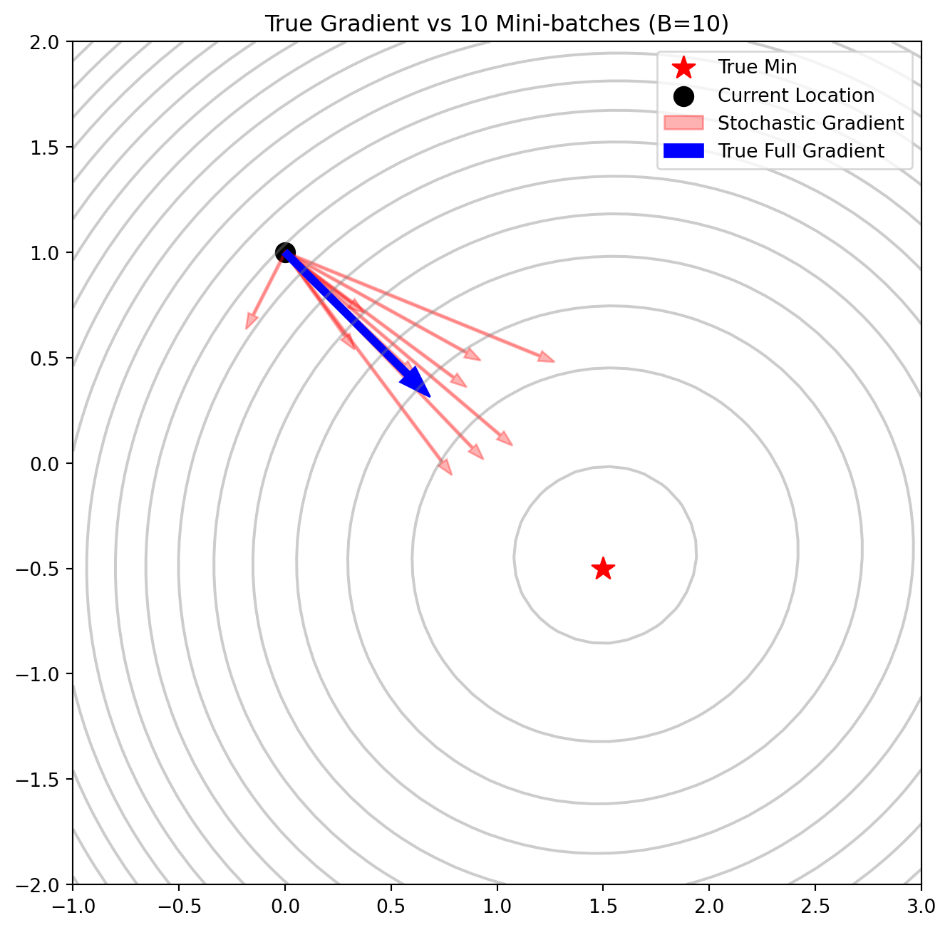
Let’s look at what this noise looks like. We will take a snapshot at a specific point on the loss surface and calculate: 1. The True Gradient (using all data). 2. Several Mini-batch Gradients (using just a few points).
Code
import numpy as npimport matplotlib.pyplot as pltnp.random.seed(42)# 1. Generate Synthetic Data (Linear Regression for simplicity)N =500X = np.random.randn(N, 2)w_true = np.array([1.5, -0.5])# y = w1*x1 + w2*x2 + noisey = X @ w_true + np.random.randn(N) *1.0# 2. Define Loss (MSE) and Gradientdef get_loss_mse(w, X_b, y_b): preds = X_b @ wreturn np.mean((preds - y_b)**2)def get_grad_mse(w, X_b, y_b):# Grad of MSE: 2/N * X.T @ (Predictions - Actuals) preds = X_b @ wreturn (2/len(y_b)) * X_b.T @ (preds - y_b)# 3. Setup Gridw1_vals = np.linspace(-1, 3, 50)w2_vals = np.linspace(-2, 2, 50)W1, W2 = np.meshgrid(w1_vals, w2_vals)Z = np.zeros_like(W1)# Calculate Full Batch Loss Surfacefor i inrange(W1.shape[0]):for j inrange(W1.shape[1]): w_curr = np.array([W1[i,j], W2[i,j]]) Z[i,j] = get_loss_mse(w_curr, X, y)# 4. Pick a test pointw_test = np.array([0.0, 1.0]) # Some point far from [1.5, -0.5]# Calculate True Gradientgrad_true = get_grad_mse(w_test, X, y)# Calculate several Mini-batch gradientsgrads_mini = []batch_size =10for k inrange(10):# Random indices idx = np.random.choice(N, batch_size, replace=False) X_b, y_b = X[idx], y[idx] g = get_grad_mse(w_test, X_b, y_b) grads_mini.append(g)# 5. Plotplt.figure(figsize=(8, 8))plt.contour(W1, W2, Z, levels=20, colors='gray', alpha=0.4)plt.scatter(w_true[0], w_true[1], c='red', marker='*', s=150, zorder=10, label="True Min")plt.scatter(w_test[0], w_test[1], c='black', s=100, label="Current Location")# Plot Mini-batch Gradients (Noisy)for i, g inenumerate(grads_mini): label ="Stochastic Gradient"if i ==0elseNone# We plot negative gradient because we move DOWNHILL plt.arrow(w_test[0], w_test[1], -g[0]*0.2, -g[1]*0.2, color='red', alpha=0.3, width=0.01, head_width=0.05, label=label)# Plot True Gradient (Correct)plt.arrow(w_test[0], w_test[1], -grad_true[0]*0.2, -grad_true[1]*0.2, color='blue', width=0.03, head_width=0.1, label="True Full Gradient")plt.title(f"True Gradient vs {len(grads_mini)} Mini-batches (B={batch_size})")plt.legend()plt.show()
Notice that the red arrows (Mini-batches) are scattered. * Some point too far left, some too far right. * However, if you averaged all the red arrows, you would get exactly the blue arrow. * The variance of the arrows represents the “Noise” in SGD.
The Drunk Walk
What happens when we actually optimize?
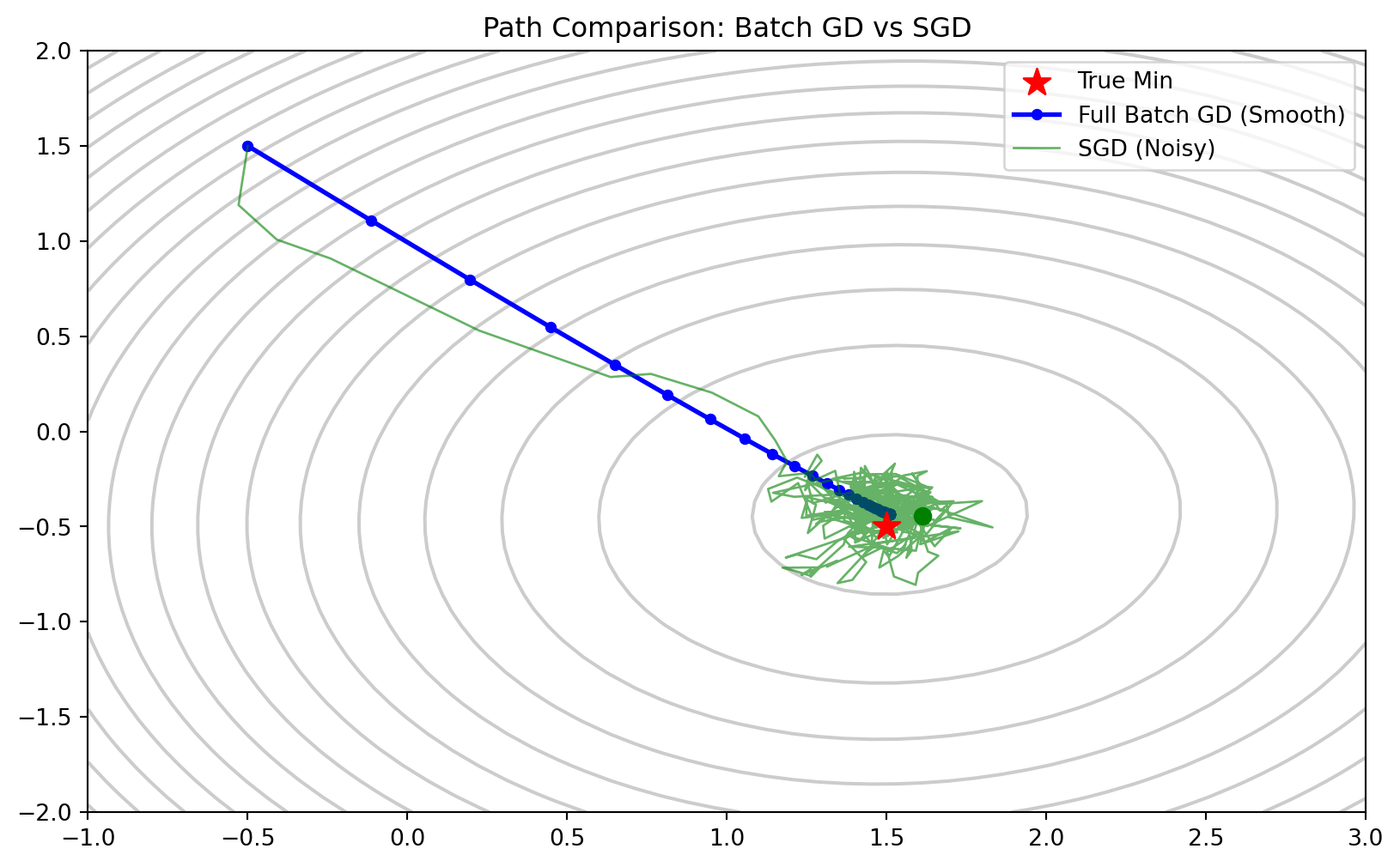
Full Batch GD: Takes a smooth, deterministic path straight to the bottom.
Stochastic Gradient Descent (SGD): Takes a jagged, wandering path.
Code
# -----------------------------# Simulation: GD vs SGD# -----------------------------# A. Full Batch Gradient Descentw_gd = np.array([-0.5, 1.5])path_gd = [w_gd.copy()]lr =0.1for i inrange(100): # 100 steps grad = get_grad_mse(w_gd, X, y) w_gd = w_gd - lr * grad path_gd.append(w_gd.copy())# B. Stochastic Gradient Descentw_sgd = np.array([-0.5, 1.5])path_sgd = [w_sgd.copy()]lr =0.1batch_size =8# We run more steps because each step is cheaperfor i inrange(400): idx = np.random.choice(N, batch_size) X_b, y_b = X[idx], y[idx] grad = get_grad_mse(w_sgd, X_b, y_b) w_sgd = w_sgd - lr * grad path_sgd.append(w_sgd.copy())# Plottingpath_gd = np.array(path_gd)path_sgd = np.array(path_sgd)plt.figure(figsize=(10, 6))plt.contour(W1, W2, Z, levels=20, colors='gray', alpha=0.4)plt.scatter(w_true[0], w_true[1], c='red', marker='*', s=150, zorder=10, label="True Min")plt.plot(path_gd[:,0], path_gd[:,1], 'o-', color='blue', label="Full Batch GD (Smooth)", linewidth=2, markersize=4)plt.plot(path_sgd[:,0], path_sgd[:,1], '-', color='green', alpha=0.6, label="SGD (Noisy)", linewidth=1)# Highlight the end of SGD to show it wobbles around the minplt.scatter(path_sgd[-1,0], path_sgd[-1,1], color='green', s=50)plt.title("Path Comparison: Batch GD vs SGD")plt.legend()plt.show()
The Trade-off
SGD is “Wiggly”: The path is not optimal. It zig-zags.
SGD is Fast: In the time it took Full Batch GD to calculate the gradient once (using 500 points), SGD could have taken \approx 60 steps (using 8 points each).
Final Convergence: Notice that SGD never completely stops. Even when it reaches the minimum, the noise keeps kicking it around. It “orbits” the minimum rather than landing on it.
This inherent noise, originally thought to be a bug, turns out to be a feature for deep learning, which we will explore in the next tab.
Summary Checklist
Method
Data per Step
Accuracy
Cost per Step
Path
Batch GD
All N
Perfect
High
Smooth
SGD
Mini-batch B
Noisy
Low
Jittery
The Epoch & The Batch
In practice, we don’t just pick random batches forever. We want to ensure we see every data point eventually. We do this by shuffling the dataset and slicing it into pieces.
Shuffle the dataset of size N.
Slice it into N/B mini-batches of size B.
Update weights for each mini-batch strictly in order.
Once all batches are done, we have completed 1 Epoch.
\text{Steps per Epoch} = \frac{N}{B}
Integrating with Previous Methods
It is crucial to understand that SGD is not a competitor to Adam or Momentum. It is the mechanism for feeding data.
Since the mini-batch gradient \nabla L_{batch} is just a vector (same shape as weights), we can plug it into any update rule we learned previously:
SGD + Momentum: Feed noisy gradients into the velocity buffer.
Adam: Feed noisy gradients into the m_t and v_t buffers.
The “Stochastic” part just refers to how we calculate \nabla L. The “Optimizer” part (Momentum/Adam) refers to how we use that \nabla L to update w.
Batch Size Impact
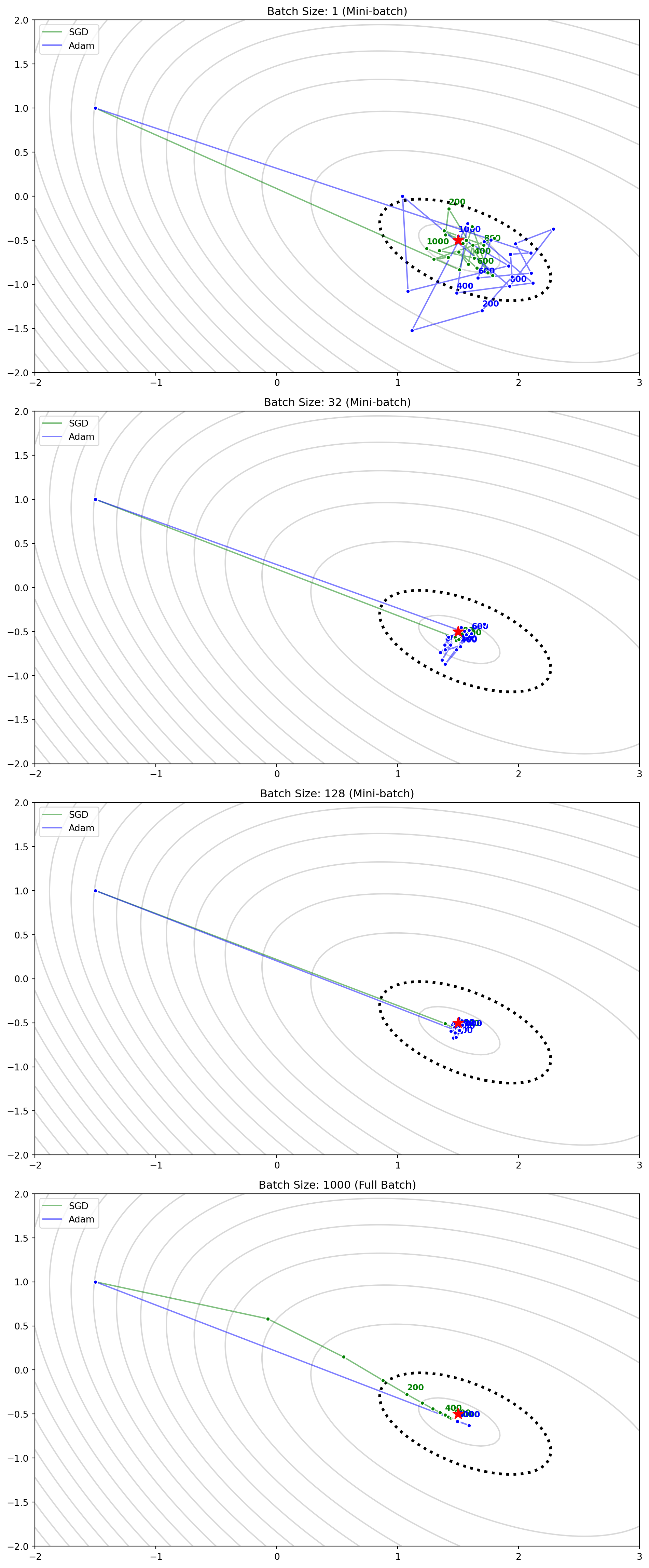
Let’s revisit our problem. We will run SGD and Adam through 4 different batch sizes, ranging from pure stochastic (B=1) to full batch (B=N).
We will use a Moderately Correlated dataset to ensure a fair test of convergence speed without the pathology of the narrow valley.
We will run each for 1,000 Epochs.
Note: For B=1, this means 1,000 \times N updates!
For Full Batch, this means 1,000 updates.
Code
import sysimport numpy as npimport timefrom IPython.display import Markdown# -----------------------------# 1. Setup Moderate Correlation Problem# -----------------------------np.random.seed(42)N_val =1000# Keeping N moderate so B=1 doesn't take forever# Generate moderate correlation (rho = 0.5)mean = [0, 0]cov = [[1, 0.5], [0.5, 1]] X_val = np.random.multivariate_normal(mean, cov, N_val)w_true_val = np.array([1.5, -0.5]) logits = X_val @ w_true_valprobs =1/ (1+ np.exp(-logits))y_val = np.random.binomial(1, probs)def get_grad_val(w, idx): X_b, y_b = X_val[idx], y_val[idx] p =1/ (1+ np.exp(-X_b @ w))# Standard Gradient g = X_b.T @ (p - y_b)# Averagereturn g /len(idx)# -----------------------------# 2. Simulation Config# -----------------------------batch_sizes = [1, 32, 128, N_val]algorithms = ["SGD", "Adam"]max_epochs =1000lr =0.1# Calculate target loss for "Vicinity"# We define "vicinity" as being within a certain loss threshold of the true minimum# Let's say loss = min_loss + 0.05p_true =1/ (1+ np.exp(-(X_val @ w_true_val)))eps =1e-12min_loss =-np.mean(y_val * np.log(p_true + eps) + (1- y_val) * np.log(1- p_true + eps))target_loss = min_loss +0.02# Define the vicinity threshold# For plotting backgroundw1_l = np.linspace(-2, 3, 100)w2_l = np.linspace(-2, 2, 100)W1_l, W2_l = np.meshgrid(w1_l, w2_l)Z_l = np.zeros_like(W1_l)for i inrange(W1_l.shape[0]):for j inrange(W1_l.shape[1]):# Full batch loss for contour p =1/ (1+ np.exp(-(X_val @ np.array([W1_l[i,j], W2_l[i,j]])))) eps =1e-12 Z_l[i,j] =-np.mean(y_val * np.log(p + eps) + (1- y_val) * np.log(1- p + eps))# Store resultsresults_batch = {} # Nested dict: batch_size -> algo -> datafig, axes = plt.subplots(len(batch_sizes), 1, figsize=(10, 24))for plot_idx, B inenumerate(batch_sizes): ax = axes[plot_idx]# Background ax.contour(W1_l, W2_l, Z_l, levels=20, colors='gray', alpha=0.3)# Add Bold Dotted Vicinity Line ax.contour(W1_l, W2_l, Z_l, levels=[target_loss], colors='black', linestyles='dotted', linewidths=3) ax.scatter(w_true_val[0], w_true_val[1], c='red', marker='*', s=150, zorder=10) ax.set_title(f"Batch Size: {B} ({'Full Batch'if B==N_val else'Mini-batch'})") results_batch[B] = {}for algo_name in algorithms: w = np.array([-1.5, 1.0]) # Start further away# State for Adam m, v =0, 0 beta1, beta2 =0.9, 0.999 t_steps =0 converged_epoch =-1# Not converged# Tracking path = [w.copy()] # Store location at end of every epoch start_time = time.time()# Epoch Loopfor epoch inrange(1, max_epochs +1):# Shuffle indices for this epoch indices = np.random.permutation(N_val)# Iteration Loop (Steps per epoch)for i inrange(0, N_val, B): idx = indices[i : min(i + B, N_val)] grad = get_grad_val(w, idx)if algo_name =="SGD": w = w - lr * gradelif algo_name =="Adam": t_steps +=1 m = beta1 * m + (1- beta1) * grad v = beta2 * v + (1- beta2) * grad**2 m_hat = m / (1- beta1**t_steps) v_hat = v / (1- beta2**t_steps) w = w - lr * m_hat / (np.sqrt(v_hat) +1e-8)# Check Vicinity Convergence# Calculate current full batch loss to see if we are in ellipse# Note: This is expensive in simulation, effectively doubling cost# In real life we calculate validation loss every epoch anywayif converged_epoch ==-1: p_curr =1/ (1+ np.exp(-(X_val @ w))) curr_loss =-np.mean(y_val * np.log(p_curr + eps) + (1- y_val) * np.log(1- p_curr + eps))if curr_loss <= target_loss: converged_epoch = epoch# End of Epoch: Record Pathif epoch %50==0: path.append(w.copy()) total_time = time.time() - start_time results_batch[B][algo_name] = {"time": total_time,"path": np.array(path),"conv_epoch": converged_epoch }# Plot Path p = np.array(path) color ='green'if algo_name =="SGD"else'blue' ax.plot(p[:,0], p[:,1], color=color, alpha=0.5, label=algo_name)# Mark every 50 epochs# Since we append to path every 50 epochs, this is just every index in p mark_indices = np.arange(0, len(p), 1) ax.scatter(p[mark_indices, 0], p[mark_indices, 1], color=color, s=20, edgecolors='white', zorder=5)# Label specific points (Every 200 epochs to avoid clutter)for mark in mark_indices: epoch_num = mark *50if epoch_num >0and epoch_num %200==0: ax.text(p[mark, 0], p[mark, 1]+0.05, f"{epoch_num}", color=color, fontsize=9, fontweight='bold') ax.legend(loc='upper left')plt.tight_layout()plt.show()# -----------------------------# 3. Create Table# -----------------------------table_md ="""| Batch Size | Algorithm | Time/Epoch (ms) | Speed to Vicinity (Epochs) ||---|---|---|---|"""for B in batch_sizes:for algo in algorithms: res = results_batch[B][algo] time_per_epoch_ms = (res['time'] / max_epochs) *1000 conv = res['conv_epoch'] if res['conv_epoch'] !=-1else"> Max" table_md +=f"| {B} | {algo} | {time_per_epoch_ms:.3f} | {conv} |\n"Markdown(table_md)
Batch Size
Algorithm
Time/Epoch (ms)
Speed to Vicinity (Epochs)
1
SGD
5.135
1
1
Adam
9.620
1
32
SGD
0.183
5
32
Adam
0.323
1
128
SGD
0.059
20
128
Adam
0.094
4
1000
SGD
0.024
156
1000
Adam
0.027
27
The results above reveal a counter-intuitive truth about training complicated ML models: Accuracy is often a waste of time.
The Computational Trade-off
Time per Epoch: You likely noticed that smaller batch sizes (e.g., B=1 or B=32) take longer per epoch.
This is due to overhead. Transferring data to the processor and launching the gradient calculation function takes fixed time. doing that 1000 times (for B=1) is slower than doing it once (for B=N).
Memory Usage: However, smaller batches use drastically less memory.
To compute a gradient, we must store the input data and the intermediate activations.
Full Batch GD requires storing the entire dataset in RAM/VRAM. For ImageNet (1M images), this is physically impossible.
Mini-batch SGD allows us to train on infinite datasets with fixed hardware.
The Convergence Surprise
Look at the “Epochs to Vicinity” column.
Full Batch GD: Takes a smooth path, but might take 100+ epochs to reach the target ellipse.
SGD (Small Batch): Reaches the target ellipse in perhaps 1-2 epochs.
Why? The answer lies in Redundancy. In any real dataset, data points are correlated. The gradient calculated from the first 32 points is likely 95% similar to the gradient calculated from the next 32 points.
Accuracy Trade-off
Smaller batch sizes lead to a larger ball around the minimum. Because SGD is random, there is noise associated with each gradient. As B \rightarrow N, this noise decreases until we reach the full batch. At the full batch, gradient descent converges pointwise.
Summary
Full Batch: Calculates the perfect gradient using all 1000 points to take 1 step.
SGD: Uses those same 1000 points to take 31 steps (roughly).
Even though the SGD steps are noisy (“drunk”), taking 31 steps in roughly the right direction gets you closer to the minimum than taking 1 perfect step.
Conclusion: We don’t need perfect gradients to learn; we just need “good enough” gradients, frequently.
Source Code
---title: "12: Stochastic Gradient Descent"format: html: code-fold: truejupyter: python3---## The Billion Row ProblemSo far, every algorithm we have looked at (Gradient Descent, Momentum, Adam, Newton) has calculated the **exact gradient**.$$ \nabla L(w) = \frac{1}{N} \sum_{i=1}^N \nabla \ell(w, x_i, y_i) $$To take **one single step**, we have to loop through every single data point in our dataset ($N$).* If $N=1,000$ (like our toy examples), this is fine.* If $N=1,000,000$ (ImageNet), this is slow.* If $N=1,000,000,000$ (Modern Large Language Models), this is impossible. You cannot wait hours just to update your weights *once*.## The Solution: Mini-BatchesWe trade **accuracy** for **speed**.Instead of calculating the gradient on the whole dataset, we select a random **Mini-batch** of size $B$ (e.g., $B=32$ or $B=64$) and calculate the gradient on that.$$ \nabla L_{batch}(w) \approx \frac{1}{B} \sum_{i \in Batch} \nabla \ell(w, x_i, y_i) $$This estimate is **noisy** (it points in a slightly wrong direction), but it is **unbiased** (on average, it points correctly) and **cheaper** to compute.---### The "Drunken" GradientLet's look at what this noise looks like. We will take a snapshot at a specific point on the loss surface and calculate:1. The **True Gradient** (using all data).2. Several **Mini-batch Gradients** (using just a few points).```{python}import numpy as npimport matplotlib.pyplot as pltnp.random.seed(42)# 1. Generate Synthetic Data (Linear Regression for simplicity)N =500X = np.random.randn(N, 2)w_true = np.array([1.5, -0.5])# y = w1*x1 + w2*x2 + noisey = X @ w_true + np.random.randn(N) *1.0# 2. Define Loss (MSE) and Gradientdef get_loss_mse(w, X_b, y_b): preds = X_b @ wreturn np.mean((preds - y_b)**2)def get_grad_mse(w, X_b, y_b):# Grad of MSE: 2/N * X.T @ (Predictions - Actuals) preds = X_b @ wreturn (2/len(y_b)) * X_b.T @ (preds - y_b)# 3. Setup Gridw1_vals = np.linspace(-1, 3, 50)w2_vals = np.linspace(-2, 2, 50)W1, W2 = np.meshgrid(w1_vals, w2_vals)Z = np.zeros_like(W1)# Calculate Full Batch Loss Surfacefor i inrange(W1.shape[0]):for j inrange(W1.shape[1]): w_curr = np.array([W1[i,j], W2[i,j]]) Z[i,j] = get_loss_mse(w_curr, X, y)# 4. Pick a test pointw_test = np.array([0.0, 1.0]) # Some point far from [1.5, -0.5]# Calculate True Gradientgrad_true = get_grad_mse(w_test, X, y)# Calculate several Mini-batch gradientsgrads_mini = []batch_size =10for k inrange(10):# Random indices idx = np.random.choice(N, batch_size, replace=False) X_b, y_b = X[idx], y[idx] g = get_grad_mse(w_test, X_b, y_b) grads_mini.append(g)# 5. Plotplt.figure(figsize=(8, 8))plt.contour(W1, W2, Z, levels=20, colors='gray', alpha=0.4)plt.scatter(w_true[0], w_true[1], c='red', marker='*', s=150, zorder=10, label="True Min")plt.scatter(w_test[0], w_test[1], c='black', s=100, label="Current Location")# Plot Mini-batch Gradients (Noisy)for i, g inenumerate(grads_mini): label ="Stochastic Gradient"if i ==0elseNone# We plot negative gradient because we move DOWNHILL plt.arrow(w_test[0], w_test[1], -g[0]*0.2, -g[1]*0.2, color='red', alpha=0.3, width=0.01, head_width=0.05, label=label)# Plot True Gradient (Correct)plt.arrow(w_test[0], w_test[1], -grad_true[0]*0.2, -grad_true[1]*0.2, color='blue', width=0.03, head_width=0.1, label="True Full Gradient")plt.title(f"True Gradient vs {len(grads_mini)} Mini-batches (B={batch_size})")plt.legend()plt.show()```Notice that the red arrows (Mini-batches) are **scattered**.* Some point too far left, some too far right.* However, if you averaged all the red arrows, you would get exactly the blue arrow.* The variance of the arrows represents the "Noise" in SGD.---### The Drunk WalkWhat happens when we actually optimize?* **Full Batch GD**: Takes a smooth, deterministic path straight to the bottom.* **Stochastic Gradient Descent (SGD)**: Takes a jagged, wandering path.```{python}# -----------------------------# Simulation: GD vs SGD# -----------------------------# A. Full Batch Gradient Descentw_gd = np.array([-0.5, 1.5])path_gd = [w_gd.copy()]lr =0.1for i inrange(100): # 100 steps grad = get_grad_mse(w_gd, X, y) w_gd = w_gd - lr * grad path_gd.append(w_gd.copy())# B. Stochastic Gradient Descentw_sgd = np.array([-0.5, 1.5])path_sgd = [w_sgd.copy()]lr =0.1batch_size =8# We run more steps because each step is cheaperfor i inrange(400): idx = np.random.choice(N, batch_size) X_b, y_b = X[idx], y[idx] grad = get_grad_mse(w_sgd, X_b, y_b) w_sgd = w_sgd - lr * grad path_sgd.append(w_sgd.copy())# Plottingpath_gd = np.array(path_gd)path_sgd = np.array(path_sgd)plt.figure(figsize=(10, 6))plt.contour(W1, W2, Z, levels=20, colors='gray', alpha=0.4)plt.scatter(w_true[0], w_true[1], c='red', marker='*', s=150, zorder=10, label="True Min")plt.plot(path_gd[:,0], path_gd[:,1], 'o-', color='blue', label="Full Batch GD (Smooth)", linewidth=2, markersize=4)plt.plot(path_sgd[:,0], path_sgd[:,1], '-', color='green', alpha=0.6, label="SGD (Noisy)", linewidth=1)# Highlight the end of SGD to show it wobbles around the minplt.scatter(path_sgd[-1,0], path_sgd[-1,1], color='green', s=50)plt.title("Path Comparison: Batch GD vs SGD")plt.legend()plt.show()```#### The Trade-off1. **SGD is "Wiggly"**: The path is not optimal. It zig-zags.2. **SGD is Fast**: In the time it took Full Batch GD to calculate the gradient *once* (using 500 points), SGD could have taken $\approx 60$ steps (using 8 points each).3. **Final Convergence**: Notice that SGD never completely stops. Even when it reaches the minimum, the noise keeps kicking it around. It "orbits" the minimum rather than landing on it.This inherent noise, originally thought to be a bug, turns out to be a **feature** for deep learning, which we will explore in the next tab.#### Summary Checklist| Method | Data per Step | Accuracy | Cost per Step | Path ||---|---|---|---|---|| **Batch GD** | All $N$ | Perfect | High | Smooth || **SGD** | Mini-batch $B$ | Noisy | Low | Jittery |### The Epoch & The BatchIn practice, we don't just pick random batches forever. We want to ensure we see *every* data point eventually. We do this by shuffling the dataset and slicing it into pieces.1. **Shuffle** the dataset of size $N$.2. **Slice** it into $N/B$ mini-batches of size $B$.3. **Update** weights for each mini-batch strictly in order.4. Once all batches are done, we have completed **1 Epoch**.$$ \text{Steps per Epoch} = \frac{N}{B} $$### Integrating with Previous MethodsIt is crucial to understand that **SGD is not a competitor to Adam or Momentum**. It is the *mechanism* for feeding data.Since the mini-batch gradient $\nabla L_{batch}$ is just a vector (same shape as weights), we can plug it into any update rule we learned previously:* **SGD + Momentum**: Feed noisy gradients into the velocity buffer.* **Adam**: Feed noisy gradients into the $m_t$ and $v_t$ buffers.The "Stochastic" part just refers to how we calculate $\nabla L$. The "Optimizer" part (Momentum/Adam) refers to how we use that $\nabla L$ to update $w$.## Batch Size ImpactLet's revisit our problem. We will run **SGD** and **Adam** through 4 different batch sizes, ranging from pure stochastic ($B=1$) to full batch ($B=N$). We will use a **Moderately Correlated** dataset to ensure a fair test of convergence speed without the pathology of the narrow valley.We will run each for **1,000 Epochs**. * Note: For $B=1$, this means $1,000 \times N$ updates!* For Full Batch, this means 1,000 updates.```{python}import sysimport numpy as npimport timefrom IPython.display import Markdown# -----------------------------# 1. Setup Moderate Correlation Problem# -----------------------------np.random.seed(42)N_val =1000# Keeping N moderate so B=1 doesn't take forever# Generate moderate correlation (rho = 0.5)mean = [0, 0]cov = [[1, 0.5], [0.5, 1]] X_val = np.random.multivariate_normal(mean, cov, N_val)w_true_val = np.array([1.5, -0.5]) logits = X_val @ w_true_valprobs =1/ (1+ np.exp(-logits))y_val = np.random.binomial(1, probs)def get_grad_val(w, idx): X_b, y_b = X_val[idx], y_val[idx] p =1/ (1+ np.exp(-X_b @ w))# Standard Gradient g = X_b.T @ (p - y_b)# Averagereturn g /len(idx)# -----------------------------# 2. Simulation Config# -----------------------------batch_sizes = [1, 32, 128, N_val]algorithms = ["SGD", "Adam"]max_epochs =1000lr =0.1# Calculate target loss for "Vicinity"# We define "vicinity" as being within a certain loss threshold of the true minimum# Let's say loss = min_loss + 0.05p_true =1/ (1+ np.exp(-(X_val @ w_true_val)))eps =1e-12min_loss =-np.mean(y_val * np.log(p_true + eps) + (1- y_val) * np.log(1- p_true + eps))target_loss = min_loss +0.02# Define the vicinity threshold# For plotting backgroundw1_l = np.linspace(-2, 3, 100)w2_l = np.linspace(-2, 2, 100)W1_l, W2_l = np.meshgrid(w1_l, w2_l)Z_l = np.zeros_like(W1_l)for i inrange(W1_l.shape[0]):for j inrange(W1_l.shape[1]):# Full batch loss for contour p =1/ (1+ np.exp(-(X_val @ np.array([W1_l[i,j], W2_l[i,j]])))) eps =1e-12 Z_l[i,j] =-np.mean(y_val * np.log(p + eps) + (1- y_val) * np.log(1- p + eps))# Store resultsresults_batch = {} # Nested dict: batch_size -> algo -> datafig, axes = plt.subplots(len(batch_sizes), 1, figsize=(10, 24))for plot_idx, B inenumerate(batch_sizes): ax = axes[plot_idx]# Background ax.contour(W1_l, W2_l, Z_l, levels=20, colors='gray', alpha=0.3)# Add Bold Dotted Vicinity Line ax.contour(W1_l, W2_l, Z_l, levels=[target_loss], colors='black', linestyles='dotted', linewidths=3) ax.scatter(w_true_val[0], w_true_val[1], c='red', marker='*', s=150, zorder=10) ax.set_title(f"Batch Size: {B} ({'Full Batch'if B==N_val else'Mini-batch'})") results_batch[B] = {}for algo_name in algorithms: w = np.array([-1.5, 1.0]) # Start further away# State for Adam m, v =0, 0 beta1, beta2 =0.9, 0.999 t_steps =0 converged_epoch =-1# Not converged# Tracking path = [w.copy()] # Store location at end of every epoch start_time = time.time()# Epoch Loopfor epoch inrange(1, max_epochs +1):# Shuffle indices for this epoch indices = np.random.permutation(N_val)# Iteration Loop (Steps per epoch)for i inrange(0, N_val, B): idx = indices[i : min(i + B, N_val)] grad = get_grad_val(w, idx)if algo_name =="SGD": w = w - lr * gradelif algo_name =="Adam": t_steps +=1 m = beta1 * m + (1- beta1) * grad v = beta2 * v + (1- beta2) * grad**2 m_hat = m / (1- beta1**t_steps) v_hat = v / (1- beta2**t_steps) w = w - lr * m_hat / (np.sqrt(v_hat) +1e-8)# Check Vicinity Convergence# Calculate current full batch loss to see if we are in ellipse# Note: This is expensive in simulation, effectively doubling cost# In real life we calculate validation loss every epoch anywayif converged_epoch ==-1: p_curr =1/ (1+ np.exp(-(X_val @ w))) curr_loss =-np.mean(y_val * np.log(p_curr + eps) + (1- y_val) * np.log(1- p_curr + eps))if curr_loss <= target_loss: converged_epoch = epoch# End of Epoch: Record Pathif epoch %50==0: path.append(w.copy()) total_time = time.time() - start_time results_batch[B][algo_name] = {"time": total_time,"path": np.array(path),"conv_epoch": converged_epoch }# Plot Path p = np.array(path) color ='green'if algo_name =="SGD"else'blue' ax.plot(p[:,0], p[:,1], color=color, alpha=0.5, label=algo_name)# Mark every 50 epochs# Since we append to path every 50 epochs, this is just every index in p mark_indices = np.arange(0, len(p), 1) ax.scatter(p[mark_indices, 0], p[mark_indices, 1], color=color, s=20, edgecolors='white', zorder=5)# Label specific points (Every 200 epochs to avoid clutter)for mark in mark_indices: epoch_num = mark *50if epoch_num >0and epoch_num %200==0: ax.text(p[mark, 0], p[mark, 1]+0.05, f"{epoch_num}", color=color, fontsize=9, fontweight='bold') ax.legend(loc='upper left')plt.tight_layout()plt.show()# -----------------------------# 3. Create Table# -----------------------------table_md ="""| Batch Size | Algorithm | Time/Epoch (ms) | Speed to Vicinity (Epochs) ||---|---|---|---|"""for B in batch_sizes:for algo in algorithms: res = results_batch[B][algo] time_per_epoch_ms = (res['time'] / max_epochs) *1000 conv = res['conv_epoch'] if res['conv_epoch'] !=-1else"> Max" table_md +=f"| {B} | {algo} | {time_per_epoch_ms:.3f} | {conv} |\n"Markdown(table_md)```The results above reveal a counter-intuitive truth about training complicated ML models: **Accuracy is often a waste of time.**### The Computational Trade-off* **Time per Epoch**: You likely noticed that smaller batch sizes (e.g., $B=1$ or $B=32$) take **longer per epoch**. * This is due to overhead. Transferring data to the processor and launching the gradient calculation function takes fixed time. doing that 1000 times (for $B=1$) is slower than doing it once (for $B=N$).* **Memory Usage**: However, smaller batches use drastically **less memory**. * To compute a gradient, we must store the input data and the intermediate activations. * Full Batch GD requires storing the entire dataset in RAM/VRAM. For ImageNet (1M images), this is physically impossible. * Mini-batch SGD allows us to train on infinite datasets with fixed hardware.### The Convergence SurpriseLook at the "Epochs to Vicinity" column.* **Full Batch GD**: Takes a smooth path, but might take 100+ epochs to reach the target ellipse.* **SGD (Small Batch)**: Reaches the target ellipse in perhaps **1-2 epochs**.**Why?**The answer lies in **Redundancy**. In any real dataset, data points are correlated. The gradient calculated from the first 32 points is likely 95% similar to the gradient calculated from the next 32 points.### Accuracy Trade-off* Smaller batch sizes lead to a larger *ball* around the minimum. Because SGD is random, there is noise associated with each gradient. As $B \rightarrow N$, this noise decreases until we reach the full batch. At the full batch, gradient descent converges pointwise.### Summary* **Full Batch**: Calculates the *perfect* gradient using all 1000 points to take **1 step**.* **SGD**: Uses those same 1000 points to take **31 steps** (roughly).Even though the SGD steps are noisy ("drunk"), taking 31 steps in roughly the right direction gets you closer to the minimum than taking 1 perfect step. > **Conclusion**: We don't need perfect gradients to learn; we just need "good enough" gradients, frequently.