In the previous tab, we saw that SGD introduces noise. Now, we ask: Where does that noise take us?
Not all minima are created equal.
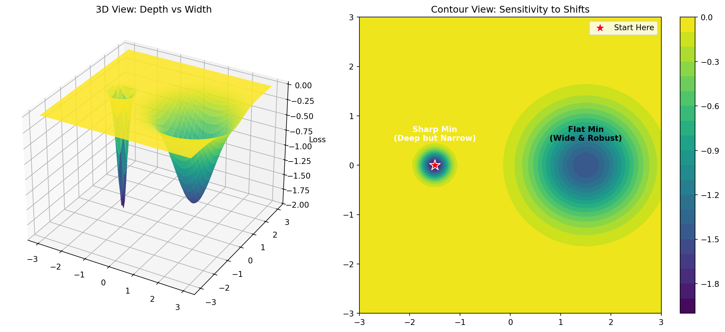
Sharp Minimum: The loss is low, but the walls are steep (High Curvature / High Hessian Trace).
Flat Minimum: The loss is low, and the region around it is wide and flat (Low Curvature / Low Hessian Trace).
The Link to Overfitting and Model Variance
Because Test Data is never identical to Training Data, we can model the transition from Train \to Test as a small perturbation \delta to our optimal weights w^*.
Sharp Minimum (High Curvature): The eigenvalues of \mathbf{H} are large. Even a tiny shift \delta results in a massive increase in error. This is High Model Variance—the model is hypersensitive to specific details of the training set (noise).
Flat Minimum (Low Curvature): The eigenvalues of \mathbf{H} are small (near zero). The term \delta^T \mathbf{H} \delta remains small. The model performance is robust to shifts. This is Low Model Variance.
Conclusion: In Deep Learning, “Overfitting” often manifests geometrically as converging to a sharp minimum. Escaping these sharp minima is equivalent to regularization.
The Non-Convex Landscape of Neural Networks
Unlike the nice bowl-shaped (convex) loss functions of Linear and Logistic Regression, Neural Networks produce highly Non-Convex landscapes filled with hills and valleys.
Why are there so many minima?
The main culprit is Symmetry. Imagine a hidden layer with 50 neurons. If you swap neuron #1 and neuron #2 (and swap their incoming/outgoing weights), the network calculates the exact same function.
Ideally, these two configurations are identical.
In parameter space, they are distinct locations w_A and w_B.
Since the loss is the same, if w_A is a minimum, w_B must also be a minimum.
For a layer with H neurons, there are H! (factorial) distinct permutations. For 50 neurons, that is \approx 10^{64} equivalent minima!
So the question isn’t “Can we find a minimum?”, but rather “Which type of minimum did we find?”
The Non-Convex Reality check
Unlike Logistic Regression (convex), Neural Networks are highly Non-Convex. This means they have thousands of different valleys (local minima).
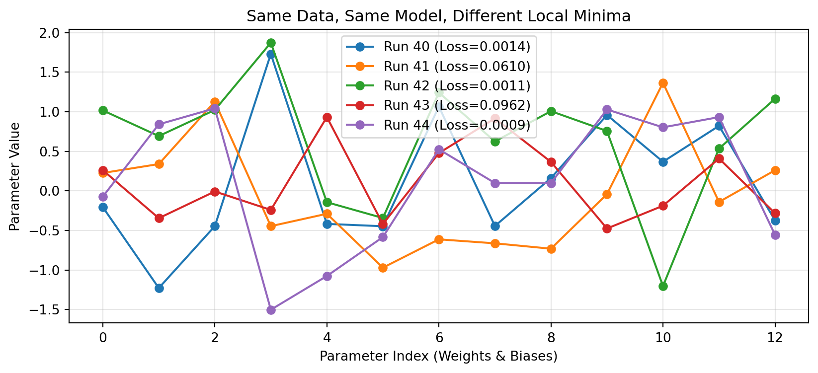
Let’s prove this numerically. We will train a simple 1-hidden-layer Neural Network on the same data 5 times, starting from different random weights.
Convex Result: All 5 runs end at the exact same w.
Non-Convex Result: All 5 runs end at different w values, even if they have the same loss!
Code
import numpy as npimport matplotlib.pyplot as plt# 1. Simple Data: y = x^2X_train = np.linspace(-1, 1, 50).reshape(-1, 1)y_train = X_train**2# 2. Define a Tiny Neural Net (Input -> 4 Hidden -> Output)def relu(x): return np.maximum(0, x)def forward(x, w1, b1, w2, b2):return relu(x @ w1 + b1) @ w2 + b2def get_loss_nn(w_flat, X, y):# Unpack weights (Input=1, Hidden=4, Output=1) w1 = w_flat[0:4].reshape(1, 4) # 4 params b1 = w_flat[4:8].reshape(1, 4) # 4 params w2 = w_flat[8:12].reshape(4, 1) # 4 params b2 = w_flat[12:13].reshape(1, 1) # 1 param preds = forward(X, w1, b1, w2, b2)return np.mean((preds - y)**2)# 3. Quick & Dirty Training Loop (Perturb & Check)def train_nn(seed): np.random.seed(seed) params = np.random.randn(13) *0.5# 13 total parameters# Simple Evolution Strategy to find a minimum current_loss = get_loss_nn(params, X_train, y_train)for i inrange(3000): # Increased steps for convergence noise = np.random.randn(13) *0.05 candidate = params + noise loss = get_loss_nn(candidate, X_train, y_train)if loss < current_loss: params = candidate current_loss = lossreturn params# 4. Helper: Numerical Hessian Approximationdef get_hessian_sharpness(w, epsilon=1e-4):# We estimate the diagonal of the Hessian (2nd derivative)# d2L/dw2 approx (L(w+e) - 2L(w) + L(w-e)) / e^2# This is a proxy for the Trace of the Hessian n_params =len(w) base_loss = get_loss_nn(w, X_train, y_train) hessian_diag_sum =0for i inrange(n_params):# Perturb parameter i w_plus = w.copy(); w_plus[i] += epsilon w_minus = w.copy(); w_minus[i] -= epsilon l_plus = get_loss_nn(w_plus, X_train, y_train) l_minus = get_loss_nn(w_minus, X_train, y_train) d2 = (l_plus -2*base_loss + l_minus) / (epsilon**2) hessian_diag_sum += d2return hessian_diag_sum # Trace Approximation# 5. Run 3 Timesfrom IPython.display import Markdownresults = []for seed in [40, 41, 42, 43, 44]: p = train_nn(seed) loss = get_loss_nn(p, X_train, y_train) sharpness = get_hessian_sharpness(p) results.append({"seed": seed, "params": p, "loss": loss, "sharpness": sharpness})# 6. Plot the Final Weightsplt.figure(figsize=(10, 4))indices = np.arange(13)for res in results: label =f"Run {res['seed']} (Loss={res['loss']:.4f})" plt.plot(indices, res['params'], 'o-', label=label)plt.title("Same Data, Same Model, Different Local Minima")plt.xlabel("Parameter Index (Weights & Biases)")plt.ylabel("Parameter Value")plt.legend()plt.grid(True, alpha=0.3)plt.show()# 7. Create Tabletable_md ="| Run | Final Loss (MSE) | Sharpness (Trace of Hessian) |\n|---|---|---|\n"for res in results: table_md +=f"| {res['seed']} | {res['loss']:.5f} | {res['sharpness']:.2f} |\n"Markdown(table_md)
Run
Final Loss (MSE)
Sharpness (Trace of Hessian)
40
0.00136
6.99
41
0.06095
3.50
42
0.00110
15.01
43
0.09618
6.87
44
0.00089
7.25
Interpreting the Trace of the Hessian
The Hessian matrix H contains all the second derivatives (curvatures) of the loss function.
Eigenvalues of H: Describe the curvature in the principal directions. Large positive eigenvalue = Steep upward curve.
Trace(H): The sum of these eigenvalues.
Think of the Trace as a “Sharpness Score”.
High Trace: The minimum is a narrow, steep pit. (Bad for generalization)
Low Trace: The minimum is a wide, gentle valley. (Good for generalization)
Key Takeaways from the Experiment
Minima are everywhere: We ran the exact same code 3 times and found 3 completely different weight vectors. If this were a simple Logistic Regression, all lines would lie perfectly on top of each other.
Loss is not enough: Look at the “Final Loss” column. All runs achieved similarly low errors (approx 0.00-0.01). To the outside world, these models perform equally well on the training set.
Sharpness Varies: Look at the “Sharpness” column. Despite having similar losses, some minima are “sharper” (higher Hessian trace) than others.
Low Sharpness (Flat): Indicates a robust solution that generalizes well.
High Sharpness (Sharp): Indicates a brittle solution prone to overfitting.
Conclusion: In Deep Learning, we don’t just want any global minimum. We want a specific kind of minimum (Flat).
Mini-Batch SGD Escapes the Sharp Trap
We would like a way to increase the chances that we end up in a flat minimum. It turns out that the noise inherent in SGD does just that!
Let’s start with a synthetic problem where we have two minima - a sharp and a flat minimum. Let’s suppose that our gradient descent routine has landed at the sharp minimum.
Code
import numpy as npimport matplotlib.pyplot as plt# Define gridx = np.linspace(-3, 3, 100)y = np.linspace(-3, 3, 100)X, Y = np.meshgrid(x, y)# Sharp Minimum at (-1.5, 0)# Deep multiplier (-2.0) and narrow spread (High coefficients like 15)Z_sharp =-2.0* np.exp(-15*(X +1.5)**2-15*Y**2)# Flat Minimum at (1.5, 0)# Shallower multiplier (-1.5) and wide spread (Low coefficients like 1)Z_flat =-1.5* np.exp(-1*(X -1.5)**2-1*Y**2)Z = Z_sharp + Z_flatfig = plt.figure(figsize=(14, 6))# Plot 1: 3D Surfaceax1 = fig.add_subplot(1, 2, 1, projection='3d')ax1.plot_surface(X, Y, Z, cmap='viridis', edgecolor='none', alpha=0.9)ax1.set_title("3D View: Depth vs Width")ax1.set_zlabel("Loss")# Plot 2: Contour Mapax2 = fig.add_subplot(1, 2, 2)contour = ax2.contourf(X, Y, Z, levels=20, cmap='viridis')plt.colorbar(contour, ax=ax2)ax2.set_title("Contour View: Sensitivity to Shifts")# Annotateax2.text(-1.5, 0.5, "Sharp Min\n(Deep but Narrow)", color='white', ha='center', fontweight='bold')ax2.text(1.5, 0.5, "Flat Min\n(Wide & Robust)", color='black', ha='center', fontweight='bold')# Add Red Star for Startax2.scatter(-1.5, 0, c='red', marker='*', s=200, edgecolors='white', zorder=10, label="Start Here")ax2.legend(loc='upper right')plt.tight_layout()plt.show()
First, let’s try Full Batch Gradient Descent (using the Adam optimizer). Since we use the full batch, the gradient is accurate. If we start deep inside the sharp hole, the gradient points strictly towards the center of the hole. There is no noise to push us out.
We will start at (-1.5, 0.0), right inside the sharp trap.
Code
import plotly.graph_objects as goimport numpy as np# 1. Define the Surface Math againdef loss_func_2d(x, y): z_sharp =-2.0* np.exp(-15*(x +1.5)**2-15*y**2) z_flat =-1.5* np.exp(-1*(x -1.5)**2-1*y**2)return z_sharp + z_flatdef grad_func_2d(x, y):# Derivative wrt x dz_dx_sharp =-2.0* np.exp(-15*(x +1.5)**2-15*y**2) * (-30*(x +1.5)) dz_dx_flat =-1.5* np.exp(-1*(x -1.5)**2-1*y**2) * (-2*(x -1.5))# Derivative wrt y dz_dy_sharp =-2.0* np.exp(-15*(x +1.5)**2-15*y**2) * (-30*y) dz_dy_flat =-1.5* np.exp(-1*(x -1.5)**2-1*y**2) * (-2*y)return np.array([dz_dx_sharp + dz_dx_flat, dz_dy_sharp + dz_dy_flat])# 2. Run Optimization (Full Batch / deterministic)w = np.array([-1.5, 0.1]) # Start slightly off-center inside the sharp holepath_x = [w[0]]path_y = [w[1]]# Adam Configm, v =0, 0beta1, beta2 =0.9, 0.999lr =0.05steps =200# REDUCED from 5000 to prevent OOM. 200 steps is plenty to show "stuck".for i inrange(1, steps+1): grad = grad_func_2d(w[0], w[1]) # Exact Gradient m = beta1 * m + (1- beta1) * grad v = beta2 * v + (1- beta2) * grad**2 m_hat = m / (1- beta1**i) v_hat = v / (1- beta2**i) w = w - lr * m_hat / (np.sqrt(v_hat) +1e-8) path_x.append(w[0]) path_y.append(w[1])# 3. Create Interactive Plotimport plotly.graph_objects as go# Contour background mathx_grid = np.linspace(-3, 3, 100)y_grid = np.linspace(-3, 3, 100)X, Y = np.meshgrid(x_grid, y_grid)Z = loss_func_2d(X, Y)frames = []for k inrange(0, len(path_x), 2): # Stride 2 frames.append(go.Frame( data=[# We only update the current DOT position go.Scatter(x=[path_x[k]], y=[path_y[k]]) ], traces=[1], # Update Trace 1 name=str(k), layout={"title": f"Full Batch Adam: Iteration {k}"} ))fig = go.Figure( data=[# Trace 0: Background Contour go.Contour( z=Z, x=x_grid, y=y_grid, colorscale='Viridis', contours=dict(start=-2, end=0, size=0.1, showlabels=False), opacity=0.6, showscale=False ),# Trace 1: The "Head" (Current Position) go.Scatter( x=[path_x[0]], y=[path_y[0]], mode='markers', marker=dict(color='blue', size=12, line=dict(width=2, color='white')), name='Current Pos' ),# Trace 2: The "Tail" (Full Path - Static Background Trace) go.Scatter( x=path_x, y=path_y, mode='lines', line=dict(color='blue', width=2, dash='dot'), opacity=0.5, name='Full Path History' ) ], frames=frames)fig.update_layout( title="Full Batch Adam: Iteration 0", xaxis=dict(range=[-3, 3], title="Parameter 1"), yaxis=dict(range=[-3, 3], scaleanchor="x", scaleratio=1), width=700, height=600, updatemenus=[dict(type="buttons", buttons=[dict( label="Play", method="animate",# KEY FIX: redraw=True allows the Title to update! args=[None, dict(frame=dict(duration=30, redraw=True), fromcurrent=True)] )] )])fig.show()
Now, let’s do the same thing with mini-batch SGD with no adaptive modifications - No momentum, no adaptive learning rates. Just gradients + noise.
In the Sharp Trap, the gradients are huge. The noise is huge. The steps are violent.
In the Flat Basin, the gradients are tiny. The noise is tiny. The steps are gentle.
Code
# 1. Define Noisy Gradientdef get_noisy_grad_2d(x, y, noise_scale=4.0): grad = grad_func_2d(x, y) noise = np.random.normal(0, noise_scale, 2)return grad + noise# 2. Run Optimization (Raw SGD)# We loop to find a representative escape pathw_final =Nonepath_x = []path_y = []# Config: High learning rate for SGD to maximize the "Kick"lr =0.1steps =1000search_limit =100for seed_attempt inrange(search_limit): np.random.seed(seed_attempt) w = np.array([-1.5, 0.1]) curr_path_x = [w[0]] curr_path_y = [w[1]]for i inrange(steps): grad = get_noisy_grad_2d(w[0], w[1], noise_scale=2.5) w = w - lr * grad # Standard SGD update curr_path_x.append(w[0]) curr_path_y.append(w[1])if w[0] >0.5: # Success check path_x = curr_path_x path_y = curr_path_yprint(f"SGD: Found escape path using seed {seed_attempt}")breakifnot path_x: path_x = curr_path_x path_y = curr_path_y# 3. Create Interactive Plotframes = []stride =10for k inrange(0, len(path_x), stride): frames.append(go.Frame( data=[go.Scatter(x=[path_x[k]], y=[path_y[k]])], traces=[1], name=str(k), layout={"title": f"Raw SGD: Iteration {k}"} ))fig = go.Figure( data=[ go.Contour( z=Z, x=x_grid, y=y_grid, colorscale='Viridis', contours=dict(start=-2, end=0, size=0.1, showlabels=False), opacity=0.6, showscale=False ), go.Scatter( x=[path_x[0]], y=[path_y[0]], mode='markers', marker=dict(color='orange', size=12, line=dict(width=2, color='white')), name='Current Pos' ), go.Scatter( x=path_x, y=path_y, mode='lines', line=dict(color='orange', width=2, dash='dot'), opacity=0.6, name='Full Path' ) ], frames=frames)fig.update_layout( title="Raw SGD: Iteration 0", xaxis=dict(range=[-3, 3]), yaxis=dict(range=[-3, 3], scaleanchor="x"), width=700, height=600, updatemenus=[dict(type="buttons", buttons=[dict(label="Play", method="animate", args=[None, dict(frame=dict(duration=30, redraw=True), fromcurrent=True)])])])fig.show()
SGD: Found escape path using seed 0
Using SGD, we escape the sharp minimum and float around the flat space until we hit the flat minimum. Unless we get really unlucky (which is a consequence of randomness), SGD will stay in this flat minimum until the end of our gradient descent routine!
The Theory: Why Noise Scales with Sharpness
You might think the noise in SGD is just random static, like a TV channel with no signal. But it is actually structured noise.
We can prove that the size of the random “kick” depends on the geometry of the valley.
1. The Step Variance
Recall the SGD step with batch size B and learning rate \eta: \Delta w = -\eta \left( \nabla L(w) + \epsilon \right)
Near a minimum, the true gradient \nabla L(w) \approx 0. So the step is dominated by the noise term -\eta \epsilon. The magnitude of this random step is determined by the trace of the Noise Covariance Matrix \Sigma:
Sharp Valley (High Tr(H)): The Temperature is hot. The steps are huge and violent. The particle ignores the barrier and jumps out.
Flat Valley (Low Tr(H)): The Temperature is cold. The steps are tiny. The particle loses energy and settles down.
This acts as an Automatic Filter: SGD implicitly performs a search where unstable (sharp) solutions are physically impossible to maintain.
Sometimes Adam Fails to Escape
Now, let’s try Stochastic Adam.
Recall that Adam divides the update by the square root of the rolling variance v_t. * In the Sharp Trap, gradients are large and noisy. This causes v_t to become very large. * The effective step size is roughly \frac{\text{gradient}}{\sqrt{\text{variance}}}.
Because Adam “normalizes” the gradients, it essentially cancels out the geometry-dependent noise! The massive kicks that allowed SGD to jump out of the hole are dampened by the variance term. Adam tries to stabilize the path, which ironically keeps it stuck in the sharp solution (or at least makes escape much harder than raw SGD).
Code
# 2. Run Optimization (Stochastic Adam)path_x = []path_y = []# Adam Config# Even with high LR, the normalization keeps steps small relative to the noise needed to jump lr =0.2beta1, beta2 =0.9, 0.999steps =1000# We use a fixed seed here. # While SGD often escapes on random seeds, Adam's normalization makes it much stickier.np.random.seed(42) w = np.array([-1.5, 0.1]) path_x = [w[0]]path_y = [w[1]]m, v =0, 0for i inrange(1, steps+1): grad = get_noisy_grad_2d(w[0], w[1], noise_scale=2.5) m = beta1 * m + (1- beta1) * grad v = beta2 * v + (1- beta2) * grad**2 m_hat = m / (1- beta1**i) v_hat = v / (1- beta2**i) w = w - lr * m_hat / (np.sqrt(v_hat) +1e-8) path_x.append(w[0]) path_y.append(w[1])# 3. Create Interactive Plotframes = []stride =10for k inrange(0, len(path_x), stride): frames.append(go.Frame( data=[go.Scatter(x=[path_x[k]], y=[path_y[k]])], traces=[1], name=str(k), layout={"title": f"Stochastic Adam: Iteration {k}"} ))fig = go.Figure( data=[ go.Contour( z=Z, x=x_grid, y=y_grid, colorscale='Viridis', contours=dict(start=-2, end=0, size=0.1, showlabels=False), opacity=0.6, showscale=False ), go.Scatter( x=[path_x[0]], y=[path_y[0]], mode='markers', marker=dict(color='purple', size=12, line=dict(width=2, color='white')), name='Current Pos' ), go.Scatter( x=path_x, y=path_y, mode='lines', line=dict(color='purple', width=2, dash='dot'), opacity=0.6, name='Full Path' ) ], frames=frames)fig.update_layout( title="Stochastic Adam: Iteration 0", xaxis=dict(range=[-3, 3]), yaxis=dict(range=[-3, 3], scaleanchor="x"), width=700, height=600, updatemenus=[dict(type="buttons", buttons=[dict(label="Play", method="animate", args=[None, dict(frame=dict(duration=30, redraw=True), fromcurrent=True)])])])fig.show()
Takeaway:
SGD: “I feel a giant gradient? I take a giant jump!” \to Escapes Trap.
Adam: “I feel a giant gradient? I’ll increase my variance counter to normalize that down.” \to Stays Stable (Stuck).
This is why, for tasks where Generalization (finding flat minima) is paramount, SGD is often preferred over Adam. However, this is a speed tradeoff since Adam can go from a bad starting location to a minimum much quicker than standard SGD. Note, though, that this example is designed to make Adam look bad - most realistic scenarios will not have large flat portions of the loss space like this and stochastic Adam will perform just fine!
The Curse of Dimensionality: Saddle Points
If you only visualize functions in 1D or 2D, you might think the biggest danger is getting stuck in “Local Minima” (small lakes higher than the ocean).
However, in High Dimensions (D=1,000,000), local minima are mathematically extremely rare.
Why?
To be a minimum, the loss function must curve UP in every single one of the 1,000,000 directions.
If there is a 50% chance of curving up or down in any random direction, the probability of a point being a minimum is (0.5)^{1,000,000} \approx 0.
Most critical points where \nabla L = 0 are actually Saddle Points: curving Up in some directions, Down in others.
The danger of Saddle Points is that Gradient Descent stalls. If you approach a saddle point along a ridge, the gradient becomes zero. The optimizer balances perfectly on the edge, unable to decide which way to fall.
Simulation: The Saddle Escape
Let’s look at a classic saddle function: f(x, y) = x^2 - y^2.
x-axis: Curves UP (Stable Ridge).
y-axis: Curves DOWN (Unstable Drop).
Point (0,0) is the saddle.
We will initialize the optimizer exactly on the ridge.
Code
# 1. Define Saddledef saddle_loss(x, y):return x**2- y**2def saddle_grad(x, y):return np.array([2*x, -2*y])# 2. Run Optimizers# A. Full Batch GD (Deterministic)# Start EXACTLY on the ridge (y=0)w_gd = np.array([-.15, 0.0]) path_gd_x = [w_gd[0]]path_gd_y = [w_gd[1]]for _ inrange(50): grad = saddle_grad(w_gd[0], w_gd[1])# The gradient wrt y is -2*0 = 0. There is NO force pushing it off the ridge! w_gd = w_gd -0.1* grad path_gd_x.append(w_gd[0]) path_gd_y.append(w_gd[1])# B. Stochastic Adam (Noisy)# Start EXACTLY on the ridge (y=0)w_adam = np.array([-.15, 0.0])path_adam_x = [w_adam[0]]path_adam_y = [w_adam[1]]# Adam Configm, v =0, 0beta1, beta2 =0.9, 0.999lr =0.1np.random.seed(42) # Ensure noise pushes us 'down' eventuallyfor i inrange(1, 51): grad_exact = saddle_grad(w_adam[0], w_adam[1])# Add small noise to simulate mini-batch variance noise = np.random.normal(0, 0.1, 2) grad = grad_exact + noise m = beta1 * m + (1- beta1) * grad v = beta2 * v + (1- beta2) * grad**2 m_hat = m / (1- beta1**i) v_hat = v / (1- beta2**i) w_adam = w_adam - lr * m_hat / (np.sqrt(v_hat) +1e-8) path_adam_x.append(w_adam[0]) path_adam_y.append(w_adam[1])# 3. Create Interactive Comparison Plot# Backgroundx_s = np.linspace(-3, 3, 50)y_s = np.linspace(-3, 3, 50)X_s, Y_s = np.meshgrid(x_s, y_s)Z_s = saddle_loss(X_s, Y_s)frames = []for k inrange(0, 50, 2): frames.append(go.Frame( data=[# Update GD Head go.Scatter(x=[path_gd_x[k]], y=[path_gd_y[k]]),# Update Adam Head go.Scatter(x=[path_adam_x[k]], y=[path_adam_y[k]]), ], traces=[1, 3], # Indices of the 'head' traces name=str(k), layout={"title": f"Saddle Point: Iteration {k}"} ))fig = go.Figure( data=[# 0. Background go.Contour( z=Z_s, x=x_s, y=y_s, colorscale='RdBu', contours=dict(start=-10, end=10, size=1.0, showlabels=False), opacity=0.5, showscale=False ),# 1. GD Head (Red) go.Scatter( x=[path_gd_x[0]], y=[path_gd_y[0]], mode='markers', marker=dict(color='red', size=12, symbol='square'), name='Full Batch GD' ),# 2. GD Path (Red Line) go.Scatter( x=path_gd_x, y=path_gd_y, mode='lines', line=dict(color='red', width=3), opacity=0.5, showlegend=False ),# 3. Adam Head (Blue) go.Scatter( x=[path_adam_x[0]], y=[path_adam_y[0]], mode='markers', marker=dict(color='blue', size=12, symbol='circle'), name='Stochastic Adam' ),# 4. Adam Path (Blue Line) go.Scatter( x=path_adam_x, y=path_adam_y, mode='lines', line=dict(color='blue', width=3), opacity=0.5, showlegend=False ) ], frames=frames)fig.update_layout( title="Saddle Point Escape: GD vs Adam", xaxis=dict(range=[-3, 3], title="Ridgeline (Stable)"), yaxis=dict(range=[-3, 3], title="Dropoff (Unstable)"), width=700, height=600, updatemenus=[dict(type="buttons", buttons=[dict(label="Play", method="animate", args=[None, dict(frame=dict(duration=50, redraw=True), fromcurrent=True)])])])fig.show()
Observation:
Full Batch GD (Red): Marches straight to (0,0) and stops. It balances perfectly on the ridge because the gradient is exactly zero in the y-direction.
Stochastic Adam (Blue): The noisy gradients act like wind. Even a tiny gust in the y-direction knocks the optimizer off balance. Once it falls off the ridge, the steep slope accelerates it away from the saddle point instantly.
In high dimensions, Stochastic methods are essential not just for speed, but for correctness - without noise, gradient descent would get stuck in the millions of saddle points that exist in neural networks.
Source Code
---title: "13: Sharp vs Flat"format: html: code-fold: truejupyter: python3---## 1. The Geometry of GeneralizationIn the previous tab, we saw that SGD introduces noise. Now, we ask: **Where does that noise take us?**Not all minima are created equal.* **Sharp Minimum**: The loss is low, but the walls are steep (High Curvature / High Hessian Trace).* **Flat Minimum**: The loss is low, and the region around it is wide and flat (Low Curvature / Low Hessian Trace).### The Link to Overfitting and Model VarianceBecause Test Data is never identical to Training Data, we can model the transition from Train $\to$ Test as a small perturbation $\delta$ to our optimal weights $w^*$.$$ \text{Loss}_{\text{test}}(w^*) \approx \text{Loss}_{\text{train}}(w^* + \delta) $$Using a Taylor Expansion around the minimum:$$ L(w^* + \delta) \approx L(w^*) + \nabla L(w^*)^T \delta + \frac{1}{2} \delta^T \mathbf{H} \delta $$Since we are at a minimum, the gradient $\nabla L(w^*) = 0$. The difference in performance is dominated by the **Hessian** $\mathbf{H}$:$$ \text{Generalization Gap} \approx \frac{1}{2} \delta^T \mathbf{H} \delta $$* **Sharp Minimum (High Curvature)**: The eigenvalues of $\mathbf{H}$ are large. Even a tiny shift $\delta$ results in a massive increase in error. This is **High Model Variance**—the model is hypersensitive to specific details of the training set (noise).* **Flat Minimum (Low Curvature)**: The eigenvalues of $\mathbf{H}$ are small (near zero). The term $\delta^T \mathbf{H} \delta$ remains small. The model performance is robust to shifts. This is **Low Model Variance**.**Conclusion**: In Deep Learning, "Overfitting" often manifests geometrically as converging to a sharp minimum. Escaping these sharp minima is equivalent to regularization.### The Non-Convex Landscape of Neural NetworksUnlike the nice bowl-shaped (convex) loss functions of Linear and Logistic Regression, Neural Networks produce highly **Non-Convex** landscapes filled with hills and valleys.**Why are there so many minima?**The main culprit is **Symmetry**. Imagine a hidden layer with 50 neurons. If you swap neuron #1 and neuron #2 (and swap their incoming/outgoing weights), the network calculates the *exact same function*. * Ideally, these two configurations are identical.* In parameter space, they are distinct locations $w_A$ and $w_B$.* Since the loss is the same, if $w_A$ is a minimum, $w_B$ must also be a minimum.* For a layer with $H$ neurons, there are $H!$ (factorial) distinct permutations. For 50 neurons, that is $\approx 10^{64}$ equivalent minima!So the question isn't "Can we find a minimum?", but rather "**Which type of minimum did we find?**"### The Non-Convex Reality checkUnlike Logistic Regression (convex), Neural Networks are highly **Non-Convex**. This means they have thousands of different valleys (local minima).Let's prove this numerically. We will train a simple 1-hidden-layer Neural Network on the same data 5 times, starting from different random weights.* **Convex Result**: All 5 runs end at the exact same $w$.* **Non-Convex Result**: All 5 runs end at different $w$ values, even if they have the same loss!```{python}import numpy as npimport matplotlib.pyplot as plt# 1. Simple Data: y = x^2X_train = np.linspace(-1, 1, 50).reshape(-1, 1)y_train = X_train**2# 2. Define a Tiny Neural Net (Input -> 4 Hidden -> Output)def relu(x): return np.maximum(0, x)def forward(x, w1, b1, w2, b2):return relu(x @ w1 + b1) @ w2 + b2def get_loss_nn(w_flat, X, y):# Unpack weights (Input=1, Hidden=4, Output=1) w1 = w_flat[0:4].reshape(1, 4) # 4 params b1 = w_flat[4:8].reshape(1, 4) # 4 params w2 = w_flat[8:12].reshape(4, 1) # 4 params b2 = w_flat[12:13].reshape(1, 1) # 1 param preds = forward(X, w1, b1, w2, b2)return np.mean((preds - y)**2)# 3. Quick & Dirty Training Loop (Perturb & Check)def train_nn(seed): np.random.seed(seed) params = np.random.randn(13) *0.5# 13 total parameters# Simple Evolution Strategy to find a minimum current_loss = get_loss_nn(params, X_train, y_train)for i inrange(3000): # Increased steps for convergence noise = np.random.randn(13) *0.05 candidate = params + noise loss = get_loss_nn(candidate, X_train, y_train)if loss < current_loss: params = candidate current_loss = lossreturn params# 4. Helper: Numerical Hessian Approximationdef get_hessian_sharpness(w, epsilon=1e-4):# We estimate the diagonal of the Hessian (2nd derivative)# d2L/dw2 approx (L(w+e) - 2L(w) + L(w-e)) / e^2# This is a proxy for the Trace of the Hessian n_params =len(w) base_loss = get_loss_nn(w, X_train, y_train) hessian_diag_sum =0for i inrange(n_params):# Perturb parameter i w_plus = w.copy(); w_plus[i] += epsilon w_minus = w.copy(); w_minus[i] -= epsilon l_plus = get_loss_nn(w_plus, X_train, y_train) l_minus = get_loss_nn(w_minus, X_train, y_train) d2 = (l_plus -2*base_loss + l_minus) / (epsilon**2) hessian_diag_sum += d2return hessian_diag_sum # Trace Approximation# 5. Run 3 Timesfrom IPython.display import Markdownresults = []for seed in [40, 41, 42, 43, 44]: p = train_nn(seed) loss = get_loss_nn(p, X_train, y_train) sharpness = get_hessian_sharpness(p) results.append({"seed": seed, "params": p, "loss": loss, "sharpness": sharpness})# 6. Plot the Final Weightsplt.figure(figsize=(10, 4))indices = np.arange(13)for res in results: label =f"Run {res['seed']} (Loss={res['loss']:.4f})" plt.plot(indices, res['params'], 'o-', label=label)plt.title("Same Data, Same Model, Different Local Minima")plt.xlabel("Parameter Index (Weights & Biases)")plt.ylabel("Parameter Value")plt.legend()plt.grid(True, alpha=0.3)plt.show()# 7. Create Tabletable_md ="| Run | Final Loss (MSE) | Sharpness (Trace of Hessian) |\n|---|---|---|\n"for res in results: table_md +=f"| {res['seed']} | {res['loss']:.5f} | {res['sharpness']:.2f} |\n"Markdown(table_md)```### Interpreting the Trace of the HessianThe Hessian matrix $H$ contains all the second derivatives (curvatures) of the loss function.* **Eigenvalues of H**: Describe the curvature in the principal directions. Large positive eigenvalue = Steep upward curve.* **Trace(H)**: The sum of these eigenvalues.Think of the Trace as a **"Sharpness Score"**.* **High Trace**: The minimum is a narrow, steep pit. (Bad for generalization)* **Low Trace**: The minimum is a wide, gentle valley. (Good for generalization)### Key Takeaways from the Experiment1. **Minima are everywhere**: We ran the exact same code 3 times and found 3 completely different weight vectors. If this were a simple Logistic Regression, all lines would lie perfectly on top of each other.2. **Loss is not enough**: Look at the "Final Loss" column. All runs achieved similarly low errors (approx 0.00-0.01). To the outside world, these models perform equally well on the training set.3. **Sharpness Varies**: Look at the "Sharpness" column. Despite having similar losses, some minima are "sharper" (higher Hessian trace) than others. * **Low Sharpness (Flat)**: Indicates a robust solution that generalizes well. * **High Sharpness (Sharp)**: Indicates a brittle solution prone to overfitting.**Conclusion**: In Deep Learning, we don't just want *any* global minimum. We want a specific *kind* of minimum (Flat).### Mini-Batch SGD Escapes the Sharp TrapWe would like a way to increase the chances that we end up in a flat minimum. It turns out that the noise inherent in SGD does just that!Let's start with a synthetic problem where we have two minima - a sharp and a flat minimum. Let's suppose that our gradient descent routine has landed at the sharp minimum.```{python}import numpy as npimport matplotlib.pyplot as plt# Define gridx = np.linspace(-3, 3, 100)y = np.linspace(-3, 3, 100)X, Y = np.meshgrid(x, y)# Sharp Minimum at (-1.5, 0)# Deep multiplier (-2.0) and narrow spread (High coefficients like 15)Z_sharp =-2.0* np.exp(-15*(X +1.5)**2-15*Y**2)# Flat Minimum at (1.5, 0)# Shallower multiplier (-1.5) and wide spread (Low coefficients like 1)Z_flat =-1.5* np.exp(-1*(X -1.5)**2-1*Y**2)Z = Z_sharp + Z_flatfig = plt.figure(figsize=(14, 6))# Plot 1: 3D Surfaceax1 = fig.add_subplot(1, 2, 1, projection='3d')ax1.plot_surface(X, Y, Z, cmap='viridis', edgecolor='none', alpha=0.9)ax1.set_title("3D View: Depth vs Width")ax1.set_zlabel("Loss")# Plot 2: Contour Mapax2 = fig.add_subplot(1, 2, 2)contour = ax2.contourf(X, Y, Z, levels=20, cmap='viridis')plt.colorbar(contour, ax=ax2)ax2.set_title("Contour View: Sensitivity to Shifts")# Annotateax2.text(-1.5, 0.5, "Sharp Min\n(Deep but Narrow)", color='white', ha='center', fontweight='bold')ax2.text(1.5, 0.5, "Flat Min\n(Wide & Robust)", color='black', ha='center', fontweight='bold')# Add Red Star for Startax2.scatter(-1.5, 0, c='red', marker='*', s=200, edgecolors='white', zorder=10, label="Start Here")ax2.legend(loc='upper right')plt.tight_layout()plt.show()```First, let's try **Full Batch Gradient Descent** (using the Adam optimizer). Since we use the full batch, the gradient is accurate. If we start deep inside the sharp hole, the gradient points strictly towards the center of the hole. There is no noise to push us out.We will start at $(-1.5, 0.0)$, right inside the sharp trap.```{python}import plotly.graph_objects as goimport numpy as np# 1. Define the Surface Math againdef loss_func_2d(x, y): z_sharp =-2.0* np.exp(-15*(x +1.5)**2-15*y**2) z_flat =-1.5* np.exp(-1*(x -1.5)**2-1*y**2)return z_sharp + z_flatdef grad_func_2d(x, y):# Derivative wrt x dz_dx_sharp =-2.0* np.exp(-15*(x +1.5)**2-15*y**2) * (-30*(x +1.5)) dz_dx_flat =-1.5* np.exp(-1*(x -1.5)**2-1*y**2) * (-2*(x -1.5))# Derivative wrt y dz_dy_sharp =-2.0* np.exp(-15*(x +1.5)**2-15*y**2) * (-30*y) dz_dy_flat =-1.5* np.exp(-1*(x -1.5)**2-1*y**2) * (-2*y)return np.array([dz_dx_sharp + dz_dx_flat, dz_dy_sharp + dz_dy_flat])# 2. Run Optimization (Full Batch / deterministic)w = np.array([-1.5, 0.1]) # Start slightly off-center inside the sharp holepath_x = [w[0]]path_y = [w[1]]# Adam Configm, v =0, 0beta1, beta2 =0.9, 0.999lr =0.05steps =200# REDUCED from 5000 to prevent OOM. 200 steps is plenty to show "stuck".for i inrange(1, steps+1): grad = grad_func_2d(w[0], w[1]) # Exact Gradient m = beta1 * m + (1- beta1) * grad v = beta2 * v + (1- beta2) * grad**2 m_hat = m / (1- beta1**i) v_hat = v / (1- beta2**i) w = w - lr * m_hat / (np.sqrt(v_hat) +1e-8) path_x.append(w[0]) path_y.append(w[1])# 3. Create Interactive Plotimport plotly.graph_objects as go# Contour background mathx_grid = np.linspace(-3, 3, 100)y_grid = np.linspace(-3, 3, 100)X, Y = np.meshgrid(x_grid, y_grid)Z = loss_func_2d(X, Y)frames = []for k inrange(0, len(path_x), 2): # Stride 2 frames.append(go.Frame( data=[# We only update the current DOT position go.Scatter(x=[path_x[k]], y=[path_y[k]]) ], traces=[1], # Update Trace 1 name=str(k), layout={"title": f"Full Batch Adam: Iteration {k}"} ))fig = go.Figure( data=[# Trace 0: Background Contour go.Contour( z=Z, x=x_grid, y=y_grid, colorscale='Viridis', contours=dict(start=-2, end=0, size=0.1, showlabels=False), opacity=0.6, showscale=False ),# Trace 1: The "Head" (Current Position) go.Scatter( x=[path_x[0]], y=[path_y[0]], mode='markers', marker=dict(color='blue', size=12, line=dict(width=2, color='white')), name='Current Pos' ),# Trace 2: The "Tail" (Full Path - Static Background Trace) go.Scatter( x=path_x, y=path_y, mode='lines', line=dict(color='blue', width=2, dash='dot'), opacity=0.5, name='Full Path History' ) ], frames=frames)fig.update_layout( title="Full Batch Adam: Iteration 0", xaxis=dict(range=[-3, 3], title="Parameter 1"), yaxis=dict(range=[-3, 3], scaleanchor="x", scaleratio=1), width=700, height=600, updatemenus=[dict(type="buttons", buttons=[dict( label="Play", method="animate",# KEY FIX: redraw=True allows the Title to update! args=[None, dict(frame=dict(duration=30, redraw=True), fromcurrent=True)] )] )])fig.show()```Now, let's do the same thing with mini-batch SGD with no adaptive modifications - No momentum, no adaptive learning rates. Just gradients + noise.* In the Sharp Trap, the gradients are huge. The noise is huge. The steps are violent.* In the Flat Basin, the gradients are tiny. The noise is tiny. The steps are gentle.```{python}# 1. Define Noisy Gradientdef get_noisy_grad_2d(x, y, noise_scale=4.0): grad = grad_func_2d(x, y) noise = np.random.normal(0, noise_scale, 2)return grad + noise# 2. Run Optimization (Raw SGD)# We loop to find a representative escape pathw_final =Nonepath_x = []path_y = []# Config: High learning rate for SGD to maximize the "Kick"lr =0.1steps =1000search_limit =100for seed_attempt inrange(search_limit): np.random.seed(seed_attempt) w = np.array([-1.5, 0.1]) curr_path_x = [w[0]] curr_path_y = [w[1]]for i inrange(steps): grad = get_noisy_grad_2d(w[0], w[1], noise_scale=2.5) w = w - lr * grad # Standard SGD update curr_path_x.append(w[0]) curr_path_y.append(w[1])if w[0] >0.5: # Success check path_x = curr_path_x path_y = curr_path_yprint(f"SGD: Found escape path using seed {seed_attempt}")breakifnot path_x: path_x = curr_path_x path_y = curr_path_y# 3. Create Interactive Plotframes = []stride =10for k inrange(0, len(path_x), stride): frames.append(go.Frame( data=[go.Scatter(x=[path_x[k]], y=[path_y[k]])], traces=[1], name=str(k), layout={"title": f"Raw SGD: Iteration {k}"} ))fig = go.Figure( data=[ go.Contour( z=Z, x=x_grid, y=y_grid, colorscale='Viridis', contours=dict(start=-2, end=0, size=0.1, showlabels=False), opacity=0.6, showscale=False ), go.Scatter( x=[path_x[0]], y=[path_y[0]], mode='markers', marker=dict(color='orange', size=12, line=dict(width=2, color='white')), name='Current Pos' ), go.Scatter( x=path_x, y=path_y, mode='lines', line=dict(color='orange', width=2, dash='dot'), opacity=0.6, name='Full Path' ) ], frames=frames)fig.update_layout( title="Raw SGD: Iteration 0", xaxis=dict(range=[-3, 3]), yaxis=dict(range=[-3, 3], scaleanchor="x"), width=700, height=600, updatemenus=[dict(type="buttons", buttons=[dict(label="Play", method="animate", args=[None, dict(frame=dict(duration=30, redraw=True), fromcurrent=True)])])])fig.show()```Using SGD, we escape the sharp minimum and float around the flat space until we hit the flat minimum. Unless we get really unlucky (which is a consequence of randomness), SGD will stay in this flat minimum until the end of our gradient descent routine!### The Theory: Why Noise Scales with SharpnessYou might think the noise in SGD is just random static, like a TV channel with no signal. But it is actually **structured noise**.We can prove that the size of the random "kick" depends on the geometry of the valley.**1. The Step Variance**Recall the SGD step with batch size $B$ and learning rate $\eta$:$$ \Delta w = -\eta \left( \nabla L(w) + \epsilon \right) $$Near a minimum, the true gradient $\nabla L(w) \approx 0$. So the step is dominated by the noise term $-\eta \epsilon$. The **magnitude** of this random step is determined by the trace of the Noise Covariance Matrix $\Sigma$:$$ E[ \|\Delta w\|^2 ] \approx \frac{\eta^2}{B} \text{Tr}(\Sigma) $$**2. Linking Noise to Curvature**For most loss functions, the variance of the gradients (Noise $\Sigma$) is roughly proportional to the squared magnitude of the gradients.Near a minimum, the gradient magnitude is determined by the **Hessian (Curvature) H**:$$ \| \nabla L(w) \| \approx \| H (w - w^*) \| $$Because of this relationship, researchers (Jastrzebski et al.) have visualized the "Temperature" of the SGD process as:$$ \text{Temperature} \propto \frac{\eta}{B} \text{Tr}(H) $$**The Result:*** **Sharp Valley (High Tr(H))**: The Temperature is hot. The steps are huge and violent. The particle ignores the barrier and jumps out.* **Flat Valley (Low Tr(H))**: The Temperature is cold. The steps are tiny. The particle loses energy and settles down.This acts as an **Automatic Filter**: SGD implicitly performs a search where unstable (sharp) solutions are physically impossible to maintain.### Sometimes Adam Fails to EscapeNow, let's try **Stochastic Adam**.Recall that Adam divides the update by the square root of the rolling variance $v_t$.* In the **Sharp Trap**, gradients are large and noisy. This causes $v_t$ to become very large.* The effective step size is roughly $\frac{\text{gradient}}{\sqrt{\text{variance}}}$.Because Adam "normalizes" the gradients, it essentially cancels out the geometry-dependent noise! The massive kicks that allowed SGD to jump out of the hole are dampened by the variance term. Adam tries to stabilize the path, which ironically keeps it stuck in the sharp solution (or at least makes escape much harder than raw SGD).```{python}# 2. Run Optimization (Stochastic Adam)path_x = []path_y = []# Adam Config# Even with high LR, the normalization keeps steps small relative to the noise needed to jump lr =0.2beta1, beta2 =0.9, 0.999steps =1000# We use a fixed seed here. # While SGD often escapes on random seeds, Adam's normalization makes it much stickier.np.random.seed(42) w = np.array([-1.5, 0.1]) path_x = [w[0]]path_y = [w[1]]m, v =0, 0for i inrange(1, steps+1): grad = get_noisy_grad_2d(w[0], w[1], noise_scale=2.5) m = beta1 * m + (1- beta1) * grad v = beta2 * v + (1- beta2) * grad**2 m_hat = m / (1- beta1**i) v_hat = v / (1- beta2**i) w = w - lr * m_hat / (np.sqrt(v_hat) +1e-8) path_x.append(w[0]) path_y.append(w[1])# 3. Create Interactive Plotframes = []stride =10for k inrange(0, len(path_x), stride): frames.append(go.Frame( data=[go.Scatter(x=[path_x[k]], y=[path_y[k]])], traces=[1], name=str(k), layout={"title": f"Stochastic Adam: Iteration {k}"} ))fig = go.Figure( data=[ go.Contour( z=Z, x=x_grid, y=y_grid, colorscale='Viridis', contours=dict(start=-2, end=0, size=0.1, showlabels=False), opacity=0.6, showscale=False ), go.Scatter( x=[path_x[0]], y=[path_y[0]], mode='markers', marker=dict(color='purple', size=12, line=dict(width=2, color='white')), name='Current Pos' ), go.Scatter( x=path_x, y=path_y, mode='lines', line=dict(color='purple', width=2, dash='dot'), opacity=0.6, name='Full Path' ) ], frames=frames)fig.update_layout( title="Stochastic Adam: Iteration 0", xaxis=dict(range=[-3, 3]), yaxis=dict(range=[-3, 3], scaleanchor="x"), width=700, height=600, updatemenus=[dict(type="buttons", buttons=[dict(label="Play", method="animate", args=[None, dict(frame=dict(duration=30, redraw=True), fromcurrent=True)])])])fig.show()```Takeaway:- **SGD**: "I feel a giant gradient? I take a giant jump!" $\to$ Escapes Trap.- **Adam**: "I feel a giant gradient? I'll increase my variance counter to normalize that down." $\to$ Stays Stable (Stuck).This is why, for tasks where Generalization (finding flat minima) is paramount, SGD is often preferred over Adam. However, this is a ***speed*** tradeoff since Adam can go from a bad starting location to a minimum much quicker than standard SGD. Note, though, that this example is designed to make Adam look bad - most realistic scenarios will not have large *flat* portions of the loss space like this and stochastic Adam will perform just fine! ## The Curse of Dimensionality: Saddle PointsIf you only visualize functions in 1D or 2D, you might think the biggest danger is getting stuck in "Local Minima" (small lakes higher than the ocean).However, in High Dimensions ($D=1,000,000$), local minima are mathematically extremely rare.**Why?**To be a minimum, the loss function must curve **UP** in every single one of the 1,000,000 directions.If there is a 50% chance of curving up or down in any random direction, the probability of a point being a minimum is $(0.5)^{1,000,000} \approx 0$.Most critical points where $\nabla L = 0$ are actually **Saddle Points**: curving Up in some directions, Down in others.The danger of Saddle Points is that **Gradient Descent stalls**. If you approach a saddle point along a ridge, the gradient becomes zero. The optimizer balances perfectly on the edge, unable to decide which way to fall.### Simulation: The Saddle EscapeLet's look at a classic saddle function: $f(x, y) = x^2 - y^2$.* $x$-axis: Curves UP (Stable Ridge).* $y$-axis: Curves DOWN (Unstable Drop).* Point $(0,0)$ is the saddle.We will initialize the optimizer **exactly** on the ridge.```{python}# 1. Define Saddledef saddle_loss(x, y):return x**2- y**2def saddle_grad(x, y):return np.array([2*x, -2*y])# 2. Run Optimizers# A. Full Batch GD (Deterministic)# Start EXACTLY on the ridge (y=0)w_gd = np.array([-.15, 0.0]) path_gd_x = [w_gd[0]]path_gd_y = [w_gd[1]]for _ inrange(50): grad = saddle_grad(w_gd[0], w_gd[1])# The gradient wrt y is -2*0 = 0. There is NO force pushing it off the ridge! w_gd = w_gd -0.1* grad path_gd_x.append(w_gd[0]) path_gd_y.append(w_gd[1])# B. Stochastic Adam (Noisy)# Start EXACTLY on the ridge (y=0)w_adam = np.array([-.15, 0.0])path_adam_x = [w_adam[0]]path_adam_y = [w_adam[1]]# Adam Configm, v =0, 0beta1, beta2 =0.9, 0.999lr =0.1np.random.seed(42) # Ensure noise pushes us 'down' eventuallyfor i inrange(1, 51): grad_exact = saddle_grad(w_adam[0], w_adam[1])# Add small noise to simulate mini-batch variance noise = np.random.normal(0, 0.1, 2) grad = grad_exact + noise m = beta1 * m + (1- beta1) * grad v = beta2 * v + (1- beta2) * grad**2 m_hat = m / (1- beta1**i) v_hat = v / (1- beta2**i) w_adam = w_adam - lr * m_hat / (np.sqrt(v_hat) +1e-8) path_adam_x.append(w_adam[0]) path_adam_y.append(w_adam[1])# 3. Create Interactive Comparison Plot# Backgroundx_s = np.linspace(-3, 3, 50)y_s = np.linspace(-3, 3, 50)X_s, Y_s = np.meshgrid(x_s, y_s)Z_s = saddle_loss(X_s, Y_s)frames = []for k inrange(0, 50, 2): frames.append(go.Frame( data=[# Update GD Head go.Scatter(x=[path_gd_x[k]], y=[path_gd_y[k]]),# Update Adam Head go.Scatter(x=[path_adam_x[k]], y=[path_adam_y[k]]), ], traces=[1, 3], # Indices of the 'head' traces name=str(k), layout={"title": f"Saddle Point: Iteration {k}"} ))fig = go.Figure( data=[# 0. Background go.Contour( z=Z_s, x=x_s, y=y_s, colorscale='RdBu', contours=dict(start=-10, end=10, size=1.0, showlabels=False), opacity=0.5, showscale=False ),# 1. GD Head (Red) go.Scatter( x=[path_gd_x[0]], y=[path_gd_y[0]], mode='markers', marker=dict(color='red', size=12, symbol='square'), name='Full Batch GD' ),# 2. GD Path (Red Line) go.Scatter( x=path_gd_x, y=path_gd_y, mode='lines', line=dict(color='red', width=3), opacity=0.5, showlegend=False ),# 3. Adam Head (Blue) go.Scatter( x=[path_adam_x[0]], y=[path_adam_y[0]], mode='markers', marker=dict(color='blue', size=12, symbol='circle'), name='Stochastic Adam' ),# 4. Adam Path (Blue Line) go.Scatter( x=path_adam_x, y=path_adam_y, mode='lines', line=dict(color='blue', width=3), opacity=0.5, showlegend=False ) ], frames=frames)fig.update_layout( title="Saddle Point Escape: GD vs Adam", xaxis=dict(range=[-3, 3], title="Ridgeline (Stable)"), yaxis=dict(range=[-3, 3], title="Dropoff (Unstable)"), width=700, height=600, updatemenus=[dict(type="buttons", buttons=[dict(label="Play", method="animate", args=[None, dict(frame=dict(duration=50, redraw=True), fromcurrent=True)])])])fig.show()```Observation:- **Full Batch GD** (Red): Marches straight to $(0,0)$ and stops. It balances perfectly on the ridge because the gradient is exactly zero in the $y$-direction.- **Stochastic Adam** (Blue): The noisy gradients act like wind. Even a tiny gust in the $y$-direction knocks the optimizer off balance. Once it falls off the ridge, the steep slope [accelerates it away from the saddle point instantly](https://youtu.be/5FjWe31S_0g?si=o4WPr3fTREGU6td7).In high dimensions, Stochastic methods are **essential** not just for speed, but for correctness - without noise, gradient descent would get stuck in the millions of saddle points that exist in neural networks.