Momentum solved the direction problem (canceling out zig-zags). However, it did not solve the scale problem.
In our “Narrow Valley” example:
The gradient for w_1 (length of valley) is tiny (\approx 0.1). We want to move fast here.
The gradient for w_2 (walls of valley) is huge (\approx 10.0). We want to move slow here.
Standard Gradient Descent uses the same learning rate \eta for both. w_{new} = w - \eta \cdot \nabla L
Newton’s Method solved this by dividing by the Hessian diagonal: w_{new} = w - \eta \cdot \frac{1}{\frac{\partial^2 L}{\partial w^2}} \cdot \nabla L This effectively gives every parameter its own custom learning rate.
Can we approximate this rescaling without calculating the expensive Hessian?
1. Fisher Information & BHHH
We can use a beautiful trick from statistical theory.
For log-likelihood functions (like cross-entropy loss), the curvature (Hessian) is related to the variance of the gradients. Specifically, under certain conditions, the Fisher Information Matrix (which approximates the Hessian) can be approximated by the outer product of the gradients:
E[\nabla L \nabla L^\top] \approx \mathbf{H}
This is known as the BHHH (Berndt-Hall-Hall-Hausman) estimator.
If we only care about the diagonal of the Hessian (ignoring interactions), we can approximate the curvature for parameter w_i simply by looking at the square of its gradient:
r_t: Accumulated squared gradients (proxy for total curvature).
\epsilon: Tiny number to avoid division by zero.
The Problem with AdaGrad
r_t keeps growing forever. As training progresses, the accumulated sum gets massive, causing the effective learning rate \frac{\eta}{\sqrt{r_t}} to shrink to zero. AdaGrad “stops learning” too early.
3. RMSProp (Root Mean Square Propagation)
Hinton (2012) proposed a fix: instead of the sum, use the exponential moving average. This allows us to “forget” ancient history.
This is RMSProp. It rescales the step size based on the recent “loudness” of the gradient.
4. Comparison: GD vs RMSProp
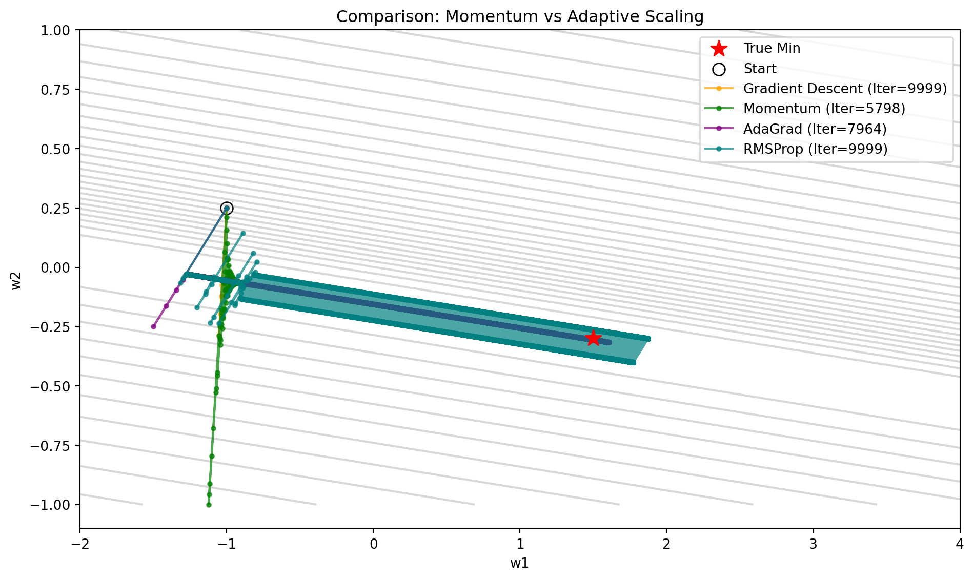
Let’s test this on our “Narrow Valley”. We expect RMSProp to normalize the valley, making the steep walls look just as flat as the valley floor.
Code
import numpy as npimport matplotlib.pyplot as pltimport timefrom IPython.display import Markdown# -----------------------------# 1. Setup the Nasty Valley # -----------------------------np.random.seed(42)n =10_000x1 = np.random.normal(0, 1, n)x2 =10.0* x1 + np.random.normal(0, .5, n) X = np.column_stack([x1, x2])w_true = np.array([1.5, -0.3]) logits = X @ w_truep =1/ (1+ np.exp(-logits))y = np.random.binomial(1, p)def get_loss(w): p =1/ (1+ np.exp(-X @ w)) eps =1e-12return-np.average(y * np.log(p + eps) + (1- y) * np.log(1- p + eps))def get_grad(w): p =1/ (1+ np.exp(-X @ w))return (X.T @ (p - y)) / n# -----------------------------# 2. Run Algorithms# -----------------------------w_start = np.array([-1.0, 0.25])tol =1e-4max_iter =10000results = []# --- A. Gradient Descent ---w = w_start.copy()path_gd = [w.copy()]start = time.time()converged =Falsefor i inrange(max_iter): grad = get_grad(w)if np.linalg.norm(grad) < tol: converged =True;break w = w -0.1* grad path_gd.append(w.copy())results.append({"name": "Gradient Descent", "path": np.array(path_gd), "time": time.time()-start, "iters": i, "conv": converged})# --- B. Momentum ---w = w_start.copy()v = np.zeros_like(w)path_mom = [w.copy()]start = time.time()converged =Falsebeta_mom =0.9for i inrange(max_iter): grad = get_grad(w)if np.linalg.norm(grad) < tol: converged =True;break v = beta_mom * v +0.1* grad w = w - v path_mom.append(w.copy())results.append({"name": "Momentum", "path": np.array(path_mom), "time": time.time()-start, "iters": i, "conv": converged})# --- C. AdaGrad ---w = w_start.copy()r = np.zeros_like(w)path_ada = [w.copy()]start = time.time()converged =Falseeta =0.5# Needs higher eta because it gets divided downfor i inrange(max_iter): grad = get_grad(w)if np.linalg.norm(grad) < tol: converged =True;break# Update accumulation r = r + grad**2# Adaptive Step# (Divide by sqrt of sum of squares) w = w - (eta / (np.sqrt(r) +1e-8)) * grad path_ada.append(w.copy())results.append({"name": "AdaGrad", "path": np.array(path_ada), "time": time.time()-start, "iters": i, "conv": converged})# --- D. RMSProp ---w = w_start.copy()r = np.zeros_like(w)path_rms = [w.copy()]start = time.time()converged =Falseeta =0.1beta =0.9for i inrange(max_iter): grad = get_grad(w)if np.linalg.norm(grad) < tol: converged =True;break# Moving Average of Squared Gradients r = beta * r + (1- beta) * grad**2# Adaptive Step w = w - (eta / (np.sqrt(r) +1e-8)) * grad path_rms.append(w.copy())results.append({"name": "RMSProp", "path": np.array(path_rms), "time": time.time()-start, "iters": i, "conv": converged})# -----------------------------# 3. Visualization# -----------------------------w1_vals = np.linspace(-2, 4, 100)w2_vals = np.linspace(-1, 1, 100)W1, W2 = np.meshgrid(w1_vals, w2_vals)Z = np.zeros_like(W1)for i inrange(W1.shape[0]):for j inrange(W1.shape[1]): Z[i,j] = get_loss(np.array([W1[i,j], W2[i,j]]))plt.figure(figsize=(10, 6))plt.contour(W1, W2, Z, levels=np.logspace(np.log10(Z.min()), np.log10(Z.max()), 30), colors='gray', alpha=0.3)plt.scatter(w_true[0], w_true[1], c='red', marker='*', s=150, zorder=10, label="True Min")plt.scatter(w_start[0], w_start[1], c='white', edgecolors='black', s=80, label="Start")colors = ['orange', 'green', 'purple', 'teal']styles = ['o-', 'o-', 'o-', 'o-']for idx, res inenumerate(results): path = res['path'] plt.plot(path[:,0], path[:,1], styles[idx], label=f"{res['name']} (Iter={res['iters']})", color=colors[idx], markersize=3, alpha=0.7, linewidth=1.5)plt.title("Comparison: Momentum vs Adaptive Scaling")plt.xlabel("w1")plt.ylabel("w2")plt.legend()plt.tight_layout()plt.show()# -----------------------------# 4. Table# -----------------------------table_md ="""| Algorithm | Iterations | Total Time (s) | Time/Iter (ms) | Final w | Status ||---|---|---|---|---|---|"""for res in results: s ="Converged ✅"if res['conv'] else"Slow ⏳" w_s =f"({res['path'][-1][0]:.3f}, {res['path'][-1][1]:.3f})" t_per = (res['time'] / res['iters']) *1000if res['iters'] >0else0 table_md +=f"| {res['name']} | {res['iters']} | {res['time']:.4f} | {t_per:.3f} | {w_s} | {s} |\n"Markdown(table_md)
Algorithm
Iterations
Total Time (s)
Time/Iter (ms)
Final w
Status
Gradient Descent
9999
0.4292
0.043
(-0.045, -0.151)
Slow ⏳
Momentum
5798
0.2183
0.038
(1.554, -0.311)
Converged ✅
AdaGrad
7964
0.3187
0.040
(1.606, -0.316)
Converged ✅
RMSProp
9999
0.5493
0.055
(1.773, -0.401)
Slow ⏳
Code
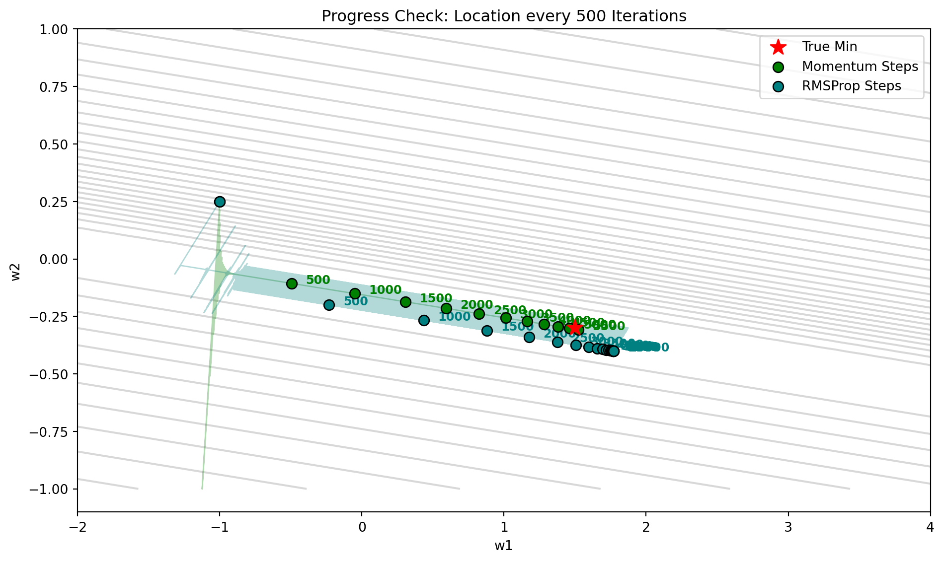
# -----------------------------# Visualization: Progress over Time# -----------------------------plt.figure(figsize=(10, 6))# Backgroundplt.contour(W1, W2, Z, levels=np.logspace(np.log10(Z.min()), np.log10(Z.max()), 30), colors='gray', alpha=0.3)plt.scatter(w_true[0], w_true[1], c='red', marker='*', s=150, zorder=10, label="True Min")selected_algos = ["Momentum", "RMSProp"]algo_colors = {"Momentum": "green", "RMSProp": "teal"}for res in results:if res['name'] notin selected_algos: continue name = res['name'] path = res['path'] col = algo_colors[name]# Plot full path faint plt.plot(path[:,0], path[:,1], color=col, alpha=0.3, linewidth=1)# Mark every 500 steps steps = np.arange(0, len(path), 500) plt.scatter(path[steps, 0], path[steps, 1], color=col, s=60, edgecolors='black', label=f"{name} Steps", zorder=5)# Annotate stepsfor step in steps:if step ==0: continue plt.text(path[step, 0]+0.1, path[step, 1], f"{step}", fontsize=9, color=col, fontweight='bold')plt.title("Progress Check: Location every 500 Iterations")plt.xlabel("w1")plt.ylabel("w2")plt.legend()plt.tight_layout()plt.show()
Key Observation: Look at the path of RMSProp (Teal). It moves almost purely vertically at first, then purely horizontally.
Why? It detects that the vertical gradient is large, so it drastically reduces the learning rate for that dimension.
It detects the horizontal gradient is small, so it boosts the learning rate for that dimension.
It essentially turns the ellipse back into a circle (locally), solving the Ill-Conditioning problem! This allows RMSProp to quickly escape the cliffs and move to the valley - about 500 iterations faster than momentum.
However, RMSprop runs into trouble when it passes the minimum - it struggles to roll backwards. This is something that momentum handles with ease!
As with most things in life, the best solution is going to be a combination of both!
Source Code
---title: "10: Adaptive Gradients"format: html: code-fold: truejupyter: python3---## The Scale ProblemMomentum solved the **direction** problem (canceling out zig-zags). However, it did not solve the **scale** problem.In our "Narrow Valley" example:- The gradient for $w_1$ (length of valley) is tiny ($\approx 0.1$). We want to move fast here.- The gradient for $w_2$ (walls of valley) is huge ($\approx 10.0$). We want to move slow here.Standard Gradient Descent uses the same learning rate $\eta$ for both.$$ w_{new} = w - \eta \cdot \nabla L $$**Newton's Method** solved this by dividing by the Hessian diagonal:$$ w_{new} = w - \eta \cdot \frac{1}{\frac{\partial^2 L}{\partial w^2}} \cdot \nabla L $$This effectively gives every parameter its own custom learning rate.Can we approximate this rescaling without calculating the expensive Hessian?---## 1. Fisher Information & BHHHWe can use a beautiful trick from statistical theory.For log-likelihood functions (like cross-entropy loss), the curvature (Hessian) is related to the variance of the gradients. Specifically, under certain conditions, the **Fisher Information Matrix** (which approximates the Hessian) can be approximated by the **outer product of the gradients**:$$ E[\nabla L \nabla L^\top] \approx \mathbf{H} $$This is known as the **BHHH (Berndt-Hall-Hall-Hausman)** estimator.If we only care about the **diagonal** of the Hessian (ignoring interactions), we can approximate the curvature for parameter $w_i$ simply by looking at the square of its gradient:$$ \frac{\partial^2 L}{\partial w_i^2} \approx \left( \frac{\partial L}{\partial w_i} \right)^2 $$This leads to the core idea of **Adaptive Gradients**:> **Divide the learning rate by the magnitude of recent gradients.**- If gradients are huge (steep walls), we divide by a huge number $\rightarrow$ **Slow down**.- If gradients are tiny (flat valley), we divide by a tiny number $\rightarrow$ **Speed up**.---## 2. AdaGrad (Adaptive Gradient)Proposed by Duchi et al. (2011), **AdaGrad** simply accumulates the sum of squared gradients over time.$$ r_{t+1} = r_t + (\nabla L)^2 $$$$ w_{t+1} = w_t - \frac{\eta}{\sqrt{r_{t+1}} + \epsilon} \odot \nabla L $$* $\odot$: Element-wise multiplication.* $r_t$: Accumulated squared gradients (proxy for total curvature).* $\epsilon$: Tiny number to avoid division by zero.### The Problem with AdaGrad$r_t$ keeps growing forever. As training progresses, the accumulated sum gets massive, causing the effective learning rate $\frac{\eta}{\sqrt{r_t}}$ to shrink to zero. AdaGrad "stops learning" too early.---## 3. RMSProp (Root Mean Square Propagation)Hinton (2012) proposed a fix: instead of the **sum**, use the **exponential moving average**. This allows us to "forget" ancient history.$$ r_{t+1} = \beta r_t + (1-\beta)(\nabla L)^2 $$$$ w_{t+1} = w_t - \frac{\eta}{\sqrt{r_{t+1}} + \epsilon} \odot \nabla L $$* $\beta$: Decay rate (typically 0.9).This is **RMSProp**. It rescales the step size based on the *recent* "loudness" of the gradient.---## 4. Comparison: GD vs RMSPropLet's test this on our "Narrow Valley". We expect RMSProp to normalize the valley, making the steep walls look just as flat as the valley floor.```{python}import numpy as npimport matplotlib.pyplot as pltimport timefrom IPython.display import Markdown# -----------------------------# 1. Setup the Nasty Valley # -----------------------------np.random.seed(42)n =10_000x1 = np.random.normal(0, 1, n)x2 =10.0* x1 + np.random.normal(0, .5, n) X = np.column_stack([x1, x2])w_true = np.array([1.5, -0.3]) logits = X @ w_truep =1/ (1+ np.exp(-logits))y = np.random.binomial(1, p)def get_loss(w): p =1/ (1+ np.exp(-X @ w)) eps =1e-12return-np.average(y * np.log(p + eps) + (1- y) * np.log(1- p + eps))def get_grad(w): p =1/ (1+ np.exp(-X @ w))return (X.T @ (p - y)) / n# -----------------------------# 2. Run Algorithms# -----------------------------w_start = np.array([-1.0, 0.25])tol =1e-4max_iter =10000results = []# --- A. Gradient Descent ---w = w_start.copy()path_gd = [w.copy()]start = time.time()converged =Falsefor i inrange(max_iter): grad = get_grad(w)if np.linalg.norm(grad) < tol: converged =True;break w = w -0.1* grad path_gd.append(w.copy())results.append({"name": "Gradient Descent", "path": np.array(path_gd), "time": time.time()-start, "iters": i, "conv": converged})# --- B. Momentum ---w = w_start.copy()v = np.zeros_like(w)path_mom = [w.copy()]start = time.time()converged =Falsebeta_mom =0.9for i inrange(max_iter): grad = get_grad(w)if np.linalg.norm(grad) < tol: converged =True;break v = beta_mom * v +0.1* grad w = w - v path_mom.append(w.copy())results.append({"name": "Momentum", "path": np.array(path_mom), "time": time.time()-start, "iters": i, "conv": converged})# --- C. AdaGrad ---w = w_start.copy()r = np.zeros_like(w)path_ada = [w.copy()]start = time.time()converged =Falseeta =0.5# Needs higher eta because it gets divided downfor i inrange(max_iter): grad = get_grad(w)if np.linalg.norm(grad) < tol: converged =True;break# Update accumulation r = r + grad**2# Adaptive Step# (Divide by sqrt of sum of squares) w = w - (eta / (np.sqrt(r) +1e-8)) * grad path_ada.append(w.copy())results.append({"name": "AdaGrad", "path": np.array(path_ada), "time": time.time()-start, "iters": i, "conv": converged})# --- D. RMSProp ---w = w_start.copy()r = np.zeros_like(w)path_rms = [w.copy()]start = time.time()converged =Falseeta =0.1beta =0.9for i inrange(max_iter): grad = get_grad(w)if np.linalg.norm(grad) < tol: converged =True;break# Moving Average of Squared Gradients r = beta * r + (1- beta) * grad**2# Adaptive Step w = w - (eta / (np.sqrt(r) +1e-8)) * grad path_rms.append(w.copy())results.append({"name": "RMSProp", "path": np.array(path_rms), "time": time.time()-start, "iters": i, "conv": converged})# -----------------------------# 3. Visualization# -----------------------------w1_vals = np.linspace(-2, 4, 100)w2_vals = np.linspace(-1, 1, 100)W1, W2 = np.meshgrid(w1_vals, w2_vals)Z = np.zeros_like(W1)for i inrange(W1.shape[0]):for j inrange(W1.shape[1]): Z[i,j] = get_loss(np.array([W1[i,j], W2[i,j]]))plt.figure(figsize=(10, 6))plt.contour(W1, W2, Z, levels=np.logspace(np.log10(Z.min()), np.log10(Z.max()), 30), colors='gray', alpha=0.3)plt.scatter(w_true[0], w_true[1], c='red', marker='*', s=150, zorder=10, label="True Min")plt.scatter(w_start[0], w_start[1], c='white', edgecolors='black', s=80, label="Start")colors = ['orange', 'green', 'purple', 'teal']styles = ['o-', 'o-', 'o-', 'o-']for idx, res inenumerate(results): path = res['path'] plt.plot(path[:,0], path[:,1], styles[idx], label=f"{res['name']} (Iter={res['iters']})", color=colors[idx], markersize=3, alpha=0.7, linewidth=1.5)plt.title("Comparison: Momentum vs Adaptive Scaling")plt.xlabel("w1")plt.ylabel("w2")plt.legend()plt.tight_layout()plt.show()# -----------------------------# 4. Table# -----------------------------table_md ="""| Algorithm | Iterations | Total Time (s) | Time/Iter (ms) | Final w | Status ||---|---|---|---|---|---|"""for res in results: s ="Converged ✅"if res['conv'] else"Slow ⏳" w_s =f"({res['path'][-1][0]:.3f}, {res['path'][-1][1]:.3f})" t_per = (res['time'] / res['iters']) *1000if res['iters'] >0else0 table_md +=f"| {res['name']} | {res['iters']} | {res['time']:.4f} | {t_per:.3f} | {w_s} | {s} |\n"Markdown(table_md)``````{python}# -----------------------------# Visualization: Progress over Time# -----------------------------plt.figure(figsize=(10, 6))# Backgroundplt.contour(W1, W2, Z, levels=np.logspace(np.log10(Z.min()), np.log10(Z.max()), 30), colors='gray', alpha=0.3)plt.scatter(w_true[0], w_true[1], c='red', marker='*', s=150, zorder=10, label="True Min")selected_algos = ["Momentum", "RMSProp"]algo_colors = {"Momentum": "green", "RMSProp": "teal"}for res in results:if res['name'] notin selected_algos: continue name = res['name'] path = res['path'] col = algo_colors[name]# Plot full path faint plt.plot(path[:,0], path[:,1], color=col, alpha=0.3, linewidth=1)# Mark every 500 steps steps = np.arange(0, len(path), 500) plt.scatter(path[steps, 0], path[steps, 1], color=col, s=60, edgecolors='black', label=f"{name} Steps", zorder=5)# Annotate stepsfor step in steps:if step ==0: continue plt.text(path[step, 0]+0.1, path[step, 1], f"{step}", fontsize=9, color=col, fontweight='bold')plt.title("Progress Check: Location every 500 Iterations")plt.xlabel("w1")plt.ylabel("w2")plt.legend()plt.tight_layout()plt.show() ```**Key Observation**: Look at the path of RMSProp (Teal). It moves almost purely vertically at first, then purely horizontally.- Why? It detects that the vertical gradient is large, so it drastically reduces the learning rate for that dimension.- It detects the horizontal gradient is small, so it boosts the learning rate for that dimension.It essentially turns the ellipse back into a circle (locally), solving the Ill-Conditioning problem! This allows RMSProp to quickly escape the cliffs and move to the valley - about 500 iterations faster than momentum.However, RMSprop runs into trouble when it **passes** the minimum - it struggles to roll backwards. This is something that momentum handles with ease! As with most things in life, the best solution is going to be a combination of both!