15: Scheduling & Convergence

Why Schedule?

In the previous tab, we learned that we often stop training early to prevent overfitting. This might lead you to ask: “If we aren’t trying to reach the absolute bottom of the loss function (the global minimum), why do we care about convergence properties? Why bother with complex Learning Rate Schedules?”

There are three key reasons:

Speed vs. Stability Paradox:
- A High Learning Rate allows us to cover distance quickly (getting to the general vicinity of the solution).
- A Low Learning Rate allows us to settle precisely into the valley floor without bouncing out.
- We need both.
The “Good” Minima are Narrow:
- Often, the solution with the best generalization isn’t just a broad bowl; it’s a specific sub-valley within that bowl.
- Constant high noise (from a constant high learning rate) might prevent the optimizer from ever “falling in” to this specific, better solution.
Modern Schedulers allow “Super-Convergence”:
- Techniques like One-Cycle Policy allow us to train models 10\times faster than standard SGD by creatively manipulating the learning rate.

Cosine Annealing

Before we look at complex policies, we must look at the “Gold Standard” default for modern training: Cosine Annealing.

In the early days of Deep Learning, people used Step Decay (dropping the learning rate by 10x every 30 epochs). This works, but it is brittle—it requires tuning exactly when to drop.

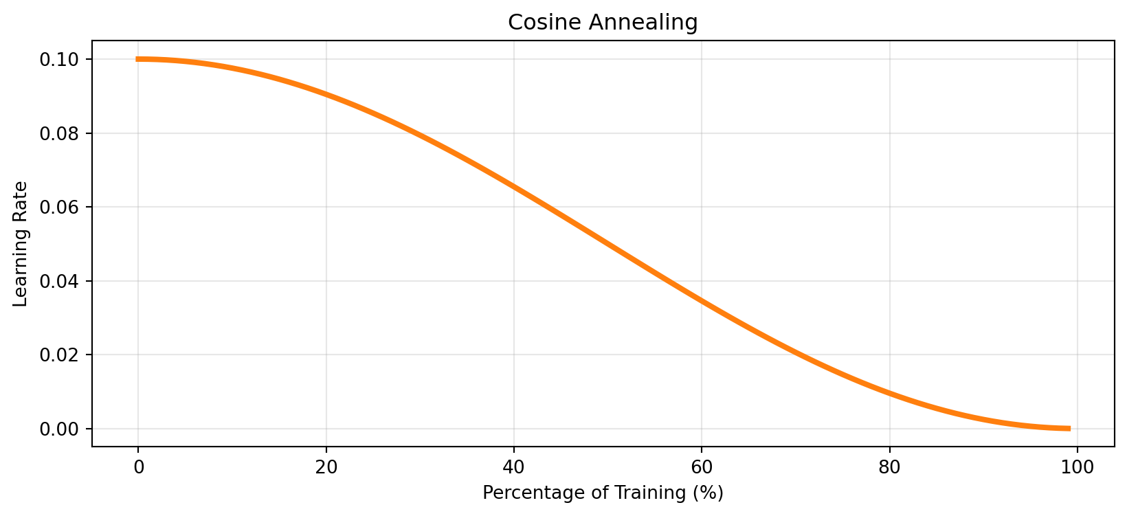
Cosine Annealing eliminates these choices. It simply follows a smooth half-cosine wave from your starting learning rate down to zero over the course of training.

Why is it so effective?

Smoothness: There are no sudden “shocks” to the optimizer that destabilize momentum.
Optimality: It spends the first half of training at a relatively high learning rate (exploring) and the second half rapidly shrinking (refining).
Simplicity: You only need to set the initial Learning Rate and the total number of Epochs. No “milestones” to guess.

Code

import numpy as np
import matplotlib.pyplot as plt

epochs = np.arange(100)
base_lr = 0.1

# Cosine Schedule Calculation
# Formula: 0.5 * lr * (1 + cos(pi * current / total))
y_cos = [base_lr * 0.5 * (1 + np.cos(np.pi * e / 100)) for e in epochs]

plt.figure(figsize=(10, 4))
plt.plot(epochs, y_cos, linewidth=3, color='tab:orange')
plt.title("Cosine Annealing")
plt.xlabel("Percentage of Training (%)")
plt.ylabel("Learning Rate")
#plt.legend()
plt.grid(True, alpha=0.3)
plt.show()

The One Cycle Policy

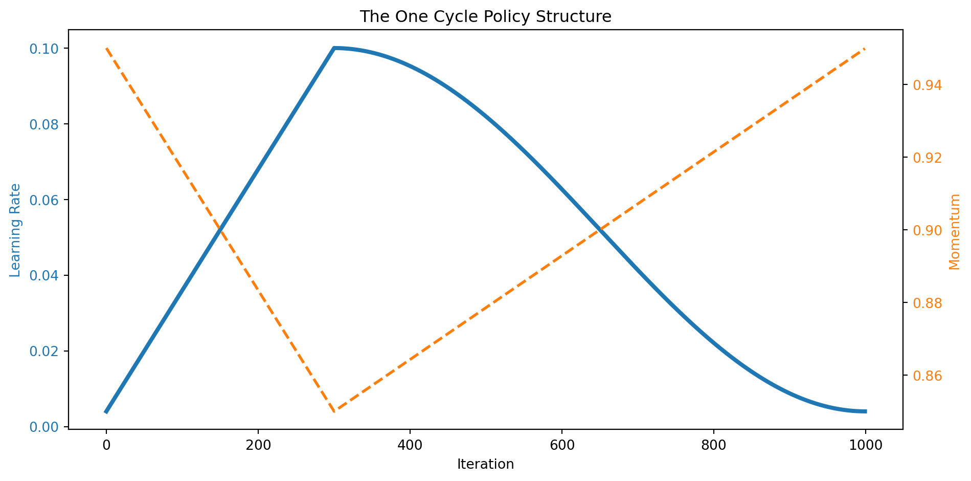
A relatively recent and powerful discovery is the One Cycle Policy (introduced by Leslie Smith). It is often used to train models significantly faster (sometimes 10\times faster) than standard schedules.

Instead of starting high and decaying (like Step or Cosine), the One Cycle policy does something counter-intuitive:

Start Low: Begin with a conservative learning rate.
Ramp Up High: Rapidly increase to a massive maximum learning rate (far higher than you would normally use).
Anneal Down: Spend the last portion of training decaying to near zero.

Why does this work?

This is related to the Sharp vs. Flat minima concept!

The massive learning rate acts as a regularizer. It prevents the model from settling into sharp, brittle local minima early in training.
It forces the optimizer to “jump over” these sharp valleys and travel across the loss landscape to find a broad, flat basin.
Once in the broad basin, the annealing allows it to settle into the center.

The Role of Momentum

In the One Cycle Policy, Momentum is famously set to move in the opposite direction of the Learning Rate (see the dashed orange line below).

Phase 1 (LR goes Up, Momentum goes Down):
- As we increase the step size, we reduce momentum.
- Since the steps are becoming huge, we don’t want the “history” of previous gradients to push us too far in the wrong direction. We want the optimizer to be agile and responsive to the current gradient.
Phase 2 (LR goes Down, Momentum goes Up):
- As we settle into the basin, the step size shrinks.
- We increase momentum to help the optimizer push through the small noise and flat regions of the valley floor without getting stuck.

Code

import numpy as np
import matplotlib.pyplot as plt

# Visualization of One Cycle Policy
total_steps = 1000
pct_start = 0.3 # 30% of time spent going UP
div_factor = 25.0
max_lr = 0.1
min_lr = max_lr / div_factor

# Simulate One Cycle Schedule
lrs_one_cycle = []
momentum_one_cycle = []

# Using PyTorch-style logic simplified
for i in range(total_steps):
    t = i / total_steps
    if t <= pct_start:
        # Phase 1: Going UP
        progress = t / pct_start
        lr = min_lr + (max_lr - min_lr) * progress
        mom = 0.95 - (0.95 - 0.85) * progress # Momentum goes DOWN as LR goes UP
    else:
        # Phase 2: Going DOWN
        progress = (t - pct_start) / (1 - pct_start)
        # Cosine decay from max_lr back to min_lr
        lr = min_lr + 0.5 * (max_lr - min_lr) * (1 + np.cos(np.pi * progress))
        mom = 0.85 + (0.95 - 0.85) * progress # Momentum goes UP as LR goes DOWN
    lrs_one_cycle.append(lr)
    momentum_one_cycle.append(mom)

fig, ax1 = plt.subplots(figsize=(10, 5))

color = 'tab:blue'
ax1.set_xlabel('Iteration')
ax1.set_ylabel('Learning Rate', color=color)
ax1.plot(lrs_one_cycle, color=color, linewidth=3, label="Learning Rate")
ax1.tick_params(axis='y', labelcolor=color)
ax1.set_title("The One Cycle Policy Structure")

ax2 = ax1.twinx()  
color = 'tab:orange'
ax2.set_ylabel('Momentum', color=color)  
ax2.plot(momentum_one_cycle, color=color, linestyle='--', linewidth=2, label="Momentum")
ax2.tick_params(axis='y', labelcolor=color)

fig.tight_layout()  
plt.show()

When to use what?

Choosing a scheduler is often as important as choosing the optimizer itself. Here are the general rules of thumb for modern Deep Learning:

1. Default Choice: Cosine Annealing

When to use: Almost always. It is the standard starting point for Image Classification, Object Detection, and general supervised tasks.
Why: It is robust. It guarantees finding a good minima if trained long enough.
Caveat: It requires you to know the total number of epochs in advance. If you change the training duration, the schedule changes shape.

2. Speed Choice: One Cycle Policy

When to use: When training time is limited, or you are “finetuning” a pre-trained model on a new dataset.
Why: It acts as a super-regularizer. The massive learning rate allows the model to traverse the loss landscape rapidly and settle into a broad basin 10x faster than constant rates.
Caveat: It is sensitive to the max_lr. If this is too high, the model diverges instantly. You often need to run a “LR Range Test” first to find the stable maximum.

3. Constant Learning Rate

When to use:
- Simpler Problems: Convex optimization or linear models where decay isn’t strictly necessary.
- Infinite Training: When training on streaming data (Reinforcement Learning) where there is no defined “end” point to decay towards.
- Adam: Sometimes Adam is smart enough to handle the decay itself (via v_t), so a simple constant LR works “good enough” for quick prototypes.

--- title: "15: Scheduling & Convergence" format: html: code-fold: true jupyter: python3 --- ## Why Schedule? In the previous tab, we learned that we often stop training early to prevent overfitting. This might lead you to ask: *"If we aren't trying to reach the absolute bottom of the loss function (the global minimum), why do we care about convergence properties? Why bother with complex Learning Rate Schedules?"* There are three key reasons: 1. **Speed vs. Stability Paradox**: * A **High Learning Rate** allows us to cover distance quickly (getting to the general vicinity of the solution). * A **Low Learning Rate** allows us to settle precisely into the valley floor without bouncing out. * We need *both*. 2. **The "Good" Minima are Narrow**: * Often, the solution with the best generalization isn't just a broad bowl; it's a specific sub-valley within that bowl. * Constant high noise (from a constant high learning rate) might prevent the optimizer from ever "falling in" to this specific, better solution. 3. **Modern Schedulers allow "Super-Convergence"**: * Techniques like **One-Cycle Policy** allow us to train models $10\times$ faster than standard SGD by creatively manipulating the learning rate. --- ## Cosine Annealing Before we look at complex policies, we must look at the "Gold Standard" default for modern training: **Cosine Annealing**. In the early days of Deep Learning, people used **Step Decay** (dropping the learning rate by 10x every 30 epochs). This works, but it is brittle—it requires tuning exactly *when* to drop. Cosine Annealing eliminates these choices. It simply follows a smooth half-cosine wave from your starting learning rate down to zero over the course of training. ### Why is it so effective? 1. **Smoothness**: There are no sudden "shocks" to the optimizer that destabilize momentum. 2. **Optimality**: It spends the first half of training at a relatively high learning rate (exploring) and the second half rapidly shrinking (refining). 3. **Simplicity**: You only need to set the initial Learning Rate and the total number of Epochs. No "milestones" to guess. ```{python} import numpy as np import matplotlib.pyplot as plt epochs = np.arange(100) base_lr = 0.1 # Cosine Schedule Calculation # Formula: 0.5 * lr * (1 + cos(pi * current / total)) y_cos = [base_lr * 0.5 * (1 + np.cos(np.pi * e / 100)) for e in epochs] plt.figure(figsize=(10, 4)) plt.plot(epochs, y_cos, linewidth=3, color='tab:orange') plt.title("Cosine Annealing") plt.xlabel("Percentage of Training (%)") plt.ylabel("Learning Rate") #plt.legend() plt.grid(True, alpha=0.3) plt.show() ``` ## The One Cycle Policy A relatively recent and powerful discovery is the **One Cycle Policy** (introduced by Leslie Smith). It is often used to train models significantly faster (sometimes $10\times$ faster) than standard schedules. Instead of starting high and decaying (like Step or Cosine), the One Cycle policy does something counter-intuitive: 1. **Start Low**: Begin with a conservative learning rate. 2. **Ramp Up High**: Rapidly increase to a massive maximum learning rate (far higher than you would normally use). 3. **Anneal Down**: Spend the last portion of training decaying to near zero. ### Why does this work? This is related to the **Sharp vs. Flat** minima concept! * The massive learning rate acts as a regularizer. It prevents the model from settling into sharp, brittle local minima early in training. * It forces the optimizer to "jump over" these sharp valleys and travel across the loss landscape to find a broad, flat basin. * Once in the broad basin, the annealing allows it to settle into the center. ### The Role of Momentum In the One Cycle Policy, **Momentum** is famously set to move in the **opposite direction** of the Learning Rate (see the dashed orange line below). 1. **Phase 1 (LR goes Up, Momentum goes Down)**: * As we increase the step size, we reduce momentum. * Since the steps are becoming huge, we don't want the "history" of previous gradients to push us too far in the wrong direction. We want the optimizer to be agile and responsive to the current gradient. 2. **Phase 2 (LR goes Down, Momentum goes Up)**: * As we settle into the basin, the step size shrinks. * We increase momentum to help the optimizer push through the small noise and flat regions of the valley floor without getting stuck. ```{python} import numpy as np import matplotlib.pyplot as plt # Visualization of One Cycle Policy total_steps = 1000 pct_start = 0.3 # 30% of time spent going UP div_factor = 25.0 max_lr = 0.1 min_lr = max_lr / div_factor # Simulate One Cycle Schedule lrs_one_cycle = [] momentum_one_cycle = [] # Using PyTorch-style logic simplified for i in range(total_steps): t = i / total_steps if t <= pct_start: # Phase 1: Going UP progress = t / pct_start lr = min_lr + (max_lr - min_lr) * progress mom = 0.95 - (0.95 - 0.85) * progress # Momentum goes DOWN as LR goes UP else: # Phase 2: Going DOWN progress = (t - pct_start) / (1 - pct_start) # Cosine decay from max_lr back to min_lr lr = min_lr + 0.5 * (max_lr - min_lr) * (1 + np.cos(np.pi * progress)) mom = 0.85 + (0.95 - 0.85) * progress # Momentum goes UP as LR goes DOWN lrs_one_cycle.append(lr) momentum_one_cycle.append(mom) fig, ax1 = plt.subplots(figsize=(10, 5)) color = 'tab:blue' ax1.set_xlabel('Iteration') ax1.set_ylabel('Learning Rate', color=color) ax1.plot(lrs_one_cycle, color=color, linewidth=3, label="Learning Rate") ax1.tick_params(axis='y', labelcolor=color) ax1.set_title("The One Cycle Policy Structure") ax2 = ax1.twinx() color = 'tab:orange' ax2.set_ylabel('Momentum', color=color) ax2.plot(momentum_one_cycle, color=color, linestyle='--', linewidth=2, label="Momentum") ax2.tick_params(axis='y', labelcolor=color) fig.tight_layout() plt.show() ``` ## When to use what? Choosing a scheduler is often as important as choosing the optimizer itself. Here are the general rules of thumb for modern Deep Learning: ### 1. Default Choice: Cosine Annealing * **When to use**: Almost always. It is the standard starting point for Image Classification, Object Detection, and general supervised tasks. * **Why**: It is robust. It guarantees finding a good minima if trained long enough. * **Caveat**: It requires you to know the total number of epochs in advance. If you change the training duration, the schedule changes shape. ### 2. Speed Choice: One Cycle Policy * **When to use**: When training time is limited, or you are "finetuning" a pre-trained model on a new dataset. * **Why**: It acts as a super-regularizer. The massive learning rate allows the model to traverse the loss landscape rapidly and settle into a broad basin 10x faster than constant rates. * **Caveat**: It is sensitive to the `max_lr`. If this is too high, the model diverges instantly. You often need to run a "LR Range Test" first to find the stable maximum. ### 3. Constant Learning Rate * **When to use**: * **Simpler Problems**: Convex optimization or linear models where decay isn't strictly necessary. * **Infinite Training**: When training on streaming data (Reinforcement Learning) where there is no defined "end" point to decay towards. * **Adam**: Sometimes Adam is smart enough to handle the decay itself (via $v_t$), so a simple constant LR works "good enough" for quick prototypes.