Nearly every model we train in this course—logistic regression, multinomial regression, neural networks, VAEs—is a composition of simple functions.
Individually, each step is easy to differentiate.
The difficulty comes from keeping track of how those steps fit together.
Computational graphs give us a systematic way to apply the chain rule to complex models.
The backward traversal of these graphs is what we call backpropagation.
The key idea of this section is simple:
Backpropagation is not a special algorithm for neural networks.
It is just the chain rule applied carefully to a graph.
The Chain Rule (revisited)
For a composition of functions
L(p(z(\mathbf{w}))),
the derivative with respect to \mathbf{w} is
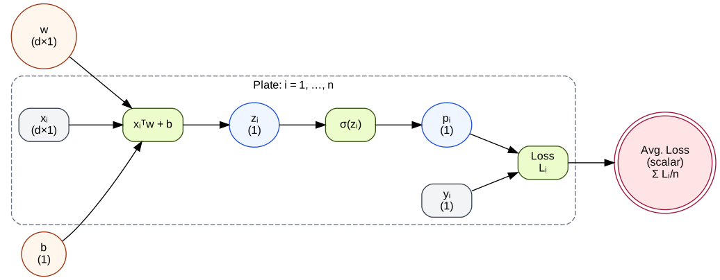
\mathbf x_i is multiplied by \mathbf w and b is added to create z_i
z_i is passed through the sigmoid function to create p_i
p_i is compared to y_i via the BCE loss to produce L_i
This construction may seem overly specified, but this is the key structure that enables computational differentiation via automatic differentiation methods!
Using the Graph To Create the Chain
Given \underset{n \times d}{\mathbf X} and a binary class vector \underset{n \times 1}{y}, logistic regression seeks to find \underset{d \times 1}{w} and \underset{1 \times 1}{b} that minimizes the total loss:
or the gradients for the unknowns are at a critical point. Additionally, we’ll need to argue that the critical points exists at a location where the Hessian is positive definite.
Unfortunately, this gradient is a little trickier than linear regression, so we’ll need to leverage the chain rule!
Because the gradient of a sum is the sum of the gradients, we can simplify this to:
\frac{1}{n}\sum \frac{\partial L_i}{\partial \mathbf w} meaning that we need to find the gradients for single instances and sum them over the loss! This is a really critical point since it means that the plate in the above graph doesn’t contribute to how we algorithmically find the gradient.
Following the Chain
Looking at the above graph, we can see that:
\mathbf x_i \rightarrow z_i \rightarrow p_i
where:
p_i = \sigma(z_i) and:
z_i = \mathbf x_i^T \mathbf w + b
This admits a chain that gives the gradients of the loss with respect to the unknowns:
An important note: the gradient for the weights, \mathbf w, and the intercept, b, share upstream terms. This means that we do not need to repeat derivations or treat each problem separately - rather, each node in the graph is associated with its own subgradient that can be reused over and over and over again. This is key for making optimization machines like PyTorch work!
Why this modular view matters
This graph-based perspective gives us three major advantages:
Reusability
Change the loss function → only the last node changes.
Extensibility
Multinomial logistic regression adds a softmax node, but the logic is identical.
Scalability
Neural networks are just deeper graphs with more nodes.
This is why modern ML libraries never “derive gradients” symbolically—they execute the graph backward.
Looking ahead
In the next section, we will:
derive the full gradient and Hessian for logistic regression,
show how we can use forward-pass and backwards-pass logic to solve the problem algorithmically
Once you are comfortable with this representation, backpropagation will feel inevitable rather than mysterious.
Key takeaways
Computational graphs turn the chain rule into a bookkeeping exercise.
The forward pass computes values; the backward pass computes gradients.
Local derivatives + shape tracking are all you need.
Backpropagation is just the chain rule applied to a graph.
Self-check questions
Draw the computational graph for
f(x) = \exp(ax + b).
What is the local derivative of the sigmoid node \frac{\partial}{\partial z}\sigma(z)?
In the logistic regression graph, which node is responsible for introducing nonlinearity to the mapping of \mathbf x_i to \hat{y_i}?
Source Code
---title: "03: Computational Graphs & Chain Rule"format: html: code-fold: truejupyter: python3---# Why this mattersNearly every model we train in this course—logistic regression, multinomial regression, neural networks, VAEs—is a **composition of simple functions**.Individually, each step is easy to differentiate. The difficulty comes from keeping track of how those steps fit together.**Computational graphs** give us a systematic way to apply the chain rule to complex models. The backward traversal of these graphs is what we call **backpropagation**.The key idea of this section is simple:> Backpropagation is not a special algorithm for neural networks.> It is just the chain rule applied carefully to a graph.---# The Chain Rule (revisited)For a composition of functions$$L(p(z(\mathbf{w}))),$$the derivative with respect to $\mathbf{w}$ is$$\frac{\partial L}{\partial \mathbf{w}}=\frac{\partial L}{\partial p}\frac{\partial p}{\partial z}\frac{\partial z}{\partial \mathbf{w}}.$$In multivariate settings, each term is:- a scalar,- a vector,- or a matrix (Jacobian),and the chain rule becomes **matrix multiplication with careful shape tracking**.Computational graphs exist to make this process mechanical.---# What is a computational graph?A computational graph is a directed acyclic graph (DAG) where:- **Nodes** are elementary operations (addition, matrix multiplication, sigmoid, log).- **Edges** carry values forward.- During differentiation, **gradients flow backward** along the same edges.There are always two passes:1. **Forward pass**: compute intermediate values.2. **Backward pass**: compute gradients using local derivatives.This separation is what allows modern ML frameworks to scale.### Node semantics: what the shapes meanIn a computational graph, **node shape is not decorative**. Each shape encodes the role a quantity plays in learning.We will use the following conventions consistently throughout the course.---#### Observed / fixed quantities (squares)```{python}from graphviz import Digraphg = Digraph( name="Observed Node",format="png", graph_attr={"bgcolor": "white"}, node_attr={"fontname": "Helvetica", "fontsize": "12"},)g.node("obs","", shape="box", style="rounded,filled", fillcolor="#f3f4f6", color="#374151",)g```Observed quantities are values provided by the dataset. They are **not optimized** and do not receive gradient updates.Examples include:- input features $\mathbf{X}$- labels $\mathbf{y}$These nodes anchor the graph to real data.---#### Learned parameters (circles)```{python}from graphviz import Digraphg = Digraph( name="Parameter Node",format="png", graph_attr={"bgcolor": "white"}, node_attr={"fontname": "Helvetica", "fontsize": "12"},)g.node("param","", shape="circle", style="filled", fillcolor="#fff7ed", color="#9a3412",)g```Learned parameters are the objects we **differentiate with respect to** and update during optimization.Examples include:- weights/coefficients $\mathbf{w}$- intercept $b$When you see a circle, you should immediately ask:> “How does the loss change if I move this parameter?”---#### Deterministic intermediate tensors (ellipses)```{python}from graphviz import Digraphg = Digraph( name="Intermediate Tensor Node",format="png", graph_attr={"bgcolor": "white"}, node_attr={"fontname": "Helvetica", "fontsize": "12"},)g.node("tensor","", shape="ellipse", style="filled", fillcolor="#eff6ff", color="#1d4ed8",)g```Intermediate tensors are values computed during the forward pass. They are **not learned directly**, but they are essential for gradient flow.Examples include:- logits $\mathbf{z}$- probabilities $\mathbf{p}$These nodes store information needed during backpropagation.---#### Operators / functions (rounded rectangles)```{python}from graphviz import Digraphg = Digraph( name="Operator Node",format="png", graph_attr={"bgcolor": "white"}, node_attr={"fontname": "Helvetica", "fontsize": "12"},)g.node("op","", shape="box", style="rounded,filled", fillcolor="#ecfccb", color="#365314",)g```Operator nodes define **how values are transformed**.Examples include:- matrix multiplication- addition- sigmoid- negative log-likelihoodEach operator node has a **local derivative** that is applied during the backward pass.---#### Scalar objectives (double circles)```{python}from graphviz import Digraphg = Digraph( name="Loss Node",format="png", graph_attr={"bgcolor": "white"}, node_attr={"fontname": "Helvetica", "fontsize": "12"},)g.node("loss","", shape="doublecircle", style="filled", fillcolor="#ffe4e6", color="#9f1239",)g```Scalar objective nodes represent quantities we aim to **minimize**.Example:- total loss $L$Backpropagation always starts here and flows backward through the graph.---Taken together, this visual language lets you identify—at a glance:- what is **observed**- what is **learned**- what is **computed**- where **gradients originate**As models grow deeper, these semantics become essential for reasoning correctly about optimization.### Plates: representing repetition and batchingMost machine learning models operate on **many independent observations**.Rather than drawing the same subgraph $n$ times, we use a **plate**.```{python}from graphviz import Digraphg = Digraph( name="Empty Plate (placeholder)",format="png", graph_attr={"bgcolor": "white", "rankdir": "LR"}, node_attr={"fontname": "Helvetica", "fontsize": "12"},)with g.subgraph(name="cluster_plate") as plate: plate.attr( label="Plate: i = 1, …, n", style="rounded,dashed", color="#6b7280", fontname="Helvetica", fontsize="12", ) plate.node("placeholder", label="(repeated subgraph goes here)", shape="plaintext", fontcolor="#9ca3af", fontsize="11", )g```A **plate** is a visual shorthand meaning:> “Everything inside this box is repeated independently for each observation.”In our setting:- Each observation $(\mathbf{x}_i, y_i)$ produces its own $z_i \rightarrow p_i \rightarrow L_i$- The **parameters** $\mathbf{w}$ and $b$ are *shared* across all observations- The **total loss** aggregates the per-observation lossesPlates are not an implementation detail. They encode an explicit modeling assumption: **observations are conditionally independent given the parameters**.---# Example: Binary Logistic Regression as a graphWe’ll start with a model you already know well.For a single observation $(\mathbf{x}_i, y_i)$:1. **Linear node** $$ z_i = \mathbf{x}_i^\top \mathbf{w} + b $$2. **Activation node** $$ p_i = \sigma(z_i) = \frac{1}{1 + e^{-z_i}} $$3. **Loss node** $$ L_i = -\big(y_i \log p_i + (1-y_i)\log(1-p_i)\big) $$Each of these is a simple function.Together, they form a computation pipeline that maps an input vector ($x_i$) to a prediction ($p_i$) that is judged against the true outcome ($y_i$)```{python}from graphviz import Digraph# Logistic regression computational graph with an observation plate.# Learned parameters (w, b) are OUTSIDE the plate (shared across all i).g = Digraph( name="Logistic Regression with Plate",format="png", graph_attr={"rankdir": "LR","bgcolor": "white","compound": "true","nodesep": "0.55","ranksep": "0.7", }, node_attr={"fontname": "Helvetica", "fontsize": "12"}, edge_attr={"fontname": "Helvetica", "fontsize": "11"},)def lab(name, shape, note=None): s =f"{name}\n({shape})"if note: s +=f"\n{note}"return s# Stylesobs =dict(shape="box", style="rounded,filled", fillcolor="#f3f4f6", color="#374151")param =dict(shape="circle", style="filled", fillcolor="#fff7ed", color="#9a3412")tensor =dict(shape="ellipse", style="filled", fillcolor="#eff6ff", color="#1d4ed8")op =dict(shape="box", style="rounded,filled", fillcolor="#ecfccb", color="#365314")loss =dict(shape="doublecircle", style="filled", fillcolor="#ffe4e6", color="#9f1239")# =========================# Shared parameters (global)# =========================g.node("w", lab("w", "d×1", ""), **param)g.node("b", lab("b", "1", ""), **param)# =========================# Observation plate# =========================with g.subgraph(name="cluster_plate") as plate: plate.attr( label="Plate: i = 1, …, n", style="rounded,dashed", color="#6b7280", fontname="Helvetica", fontsize="12", ) plate.node("x_i", lab("xᵢ", "d×1", ""), **obs) plate.node("y_i", lab("yᵢ", "1", ""), **obs) plate.node("lin_i", "xᵢᵀw + b", **op) plate.node("z_i", lab("zᵢ", "1", ""), **tensor) plate.node("sig_i", "σ(zᵢ)", **op) plate.node("p_i", lab("pᵢ", "1", ""), **tensor) plate.node("ell_i", "Loss\nLᵢ", **op) plate.edge("x_i", "lin_i") plate.edge("lin_i", "z_i") plate.edge("z_i", "sig_i") plate.edge("sig_i", "p_i") plate.edge("p_i", "ell_i") plate.edge("y_i", "ell_i")# =========================# Total loss# =========================g.node("L", lab("Avg. Loss", "scalar", "Σ Lᵢ/n"), **loss)# IMPORTANT FIX:# Draw edges directly to lin_i (no lhead)g.edge("w", "lin_i")g.edge("b", "lin_i")g.edge("ell_i", "L")g```1. $\mathbf x_i$ is multiplied by $\mathbf w$ and $b$ is added to create $z_i$2. $z_i$ is passed through the sigmoid function to create $p_i$3. $p_i$ is compared to $y_i$ via the BCE loss to produce $L_i$This construction may seem overly specified, but this is the **key** structure that enables ***computational differentiation*** via automatic differentiation methods!# Using the Graph To Create the ChainGiven $\underset{n \times d}{\mathbf X}$ and a binary class vector $\underset{n \times 1}{y}$, logistic regression seeks to find $\underset{d \times 1}{w}$ and $\underset{1 \times 1}{b}$ that minimizes the total loss:$$\underset{\{\mathbf w, b\}}{\min} \frac{1}{n}\sum \limits_{i = 1}^n -\big(y_i \log p_i + (1-y_i)\log(1-p_i)\big)$$We know that this minimum is achieved where:$$\frac{\partial L}{\partial \mathbf w} = \mathbf 0 \text{ ; } \frac{\partial L}{\partial b} = 0$$or the **gradients** for the unknowns are at a critical point. Additionally, we'll need to argue that the critical points exists at a location where the **Hessian** is positive definite. Unfortunately, this gradient is a little trickier than linear regression, so we'll need to leverage the chain rule!### The loss stepWe'll start by making the observation that:$$\frac{\partial L}{\partial \mathbf w} = \frac{\partial \frac{1}{n}\sum L_i}{\partial \mathbf w}$$Because the gradient of a sum is the sum of the gradients, we can simplify this to:$$\frac{1}{n}\sum \frac{\partial L_i}{\partial \mathbf w} $$meaning that we need to find the gradients for single instances and sum them over the loss! This is a **really critical point** since it means that the plate in the above graph doesn't contribute to how we algorithmically find the gradient.### Following the ChainLooking at the above graph, we can see that:$$\mathbf x_i \rightarrow z_i \rightarrow p_i$$ where:$$p_i = \sigma(z_i)$$and:$$z_i = \mathbf x_i^T \mathbf w + b$$This admits a chain that gives the gradients of the loss with respect to the unknowns:$$\frac{\partial L_i}{\partial \mathbf w} = \frac{\partial L_i}{\partial p_i}\frac{\partial p_i}{\partial z_i}\frac{\partial z_i}{\partial \mathbf w}$$$$\frac{\partial L_i}{\partial b} = \frac{\partial L_i}{\partial p_i}\frac{\partial p_i}{\partial z_i}\frac{\partial z_i}{\partial b}$$Easy-peasy!An important note: the gradient for the weights, $\mathbf w$, and the intercept, $b$, **share upstream terms**. This means that we do not need to repeat derivations or treat each problem separately - rather, each node in the graph is associated with its own subgradient that can be reused over and over and over again. This is **key** for making optimization machines like PyTorch work!---# Why this modular view mattersThis graph-based perspective gives us three major advantages:1. **Reusability** Change the loss function → only the last node changes.2. **Extensibility** Multinomial logistic regression adds a softmax node, but the logic is identical.3. **Scalability** Neural networks are just deeper graphs with more nodes.This is why modern ML libraries never “derive gradients” symbolically—they **execute the graph backward**.---# Looking aheadIn the next section, we will:- derive the full gradient and Hessian for logistic regression,- show how we can use **forward-pass** and **backwards-pass** logic to solve the problem algorithmicallyOnce you are comfortable with this representation, backpropagation will feel inevitable rather than mysterious.---# Key takeaways- Computational graphs turn the chain rule into a bookkeeping exercise.- The forward pass computes values; the backward pass computes gradients.- Local derivatives + shape tracking are all you need.- Backpropagation is just the chain rule applied to a graph.---# Self-check questions1. Draw the computational graph for $$ f(x) = \exp(ax + b). $$2. What is the local derivative of the sigmoid node $\frac{\partial}{\partial z}\sigma(z)$?3. In the logistic regression graph, which node is responsible for introducing nonlinearity to the mapping of $\mathbf x_i$ to $\hat{y_i}$?