In the previous section, we saw that standard Gradient Descent fails when the loss landscape is “ill-conditioned”—shaped like a narrow taco or a long canyon.
This happens because GD is isotropic: it treats every direction in parameter space the same.
It sees a steep slope (the canyon walls) and thinks “I should take a big step this way.”
It sees a flat slope (the valley floor) and thinks “I should take a tiny step this way.”
This is exactly the opposite of what we want. We want to move cautiously in steep directions and aggressively in flat directions.
Newton’s Method solves this by using curvature information (second derivatives) to measure the shape of the landscape and correct the step size for every direction individually.
1. The Geometry of Curvature
We previously defined the Gradient \nabla L (slope). Now we stick with the Hessian \mathbf H (curvature).
For a function with two parameters w_1, w_2, the Hessian is the 2 \times 2 matrix of second derivatives:
Newton: \mathbf w_{new} = \mathbf w - \eta \mathbf H^{-1} \nabla L
The difference is the Inverse Hessian\mathbf H^{-1}.
Note: While Newton updates do not require a step size (e.g. \eta = 1), it is often advised to introduce one to dampen the Newton updates at the original “bad” starting points.
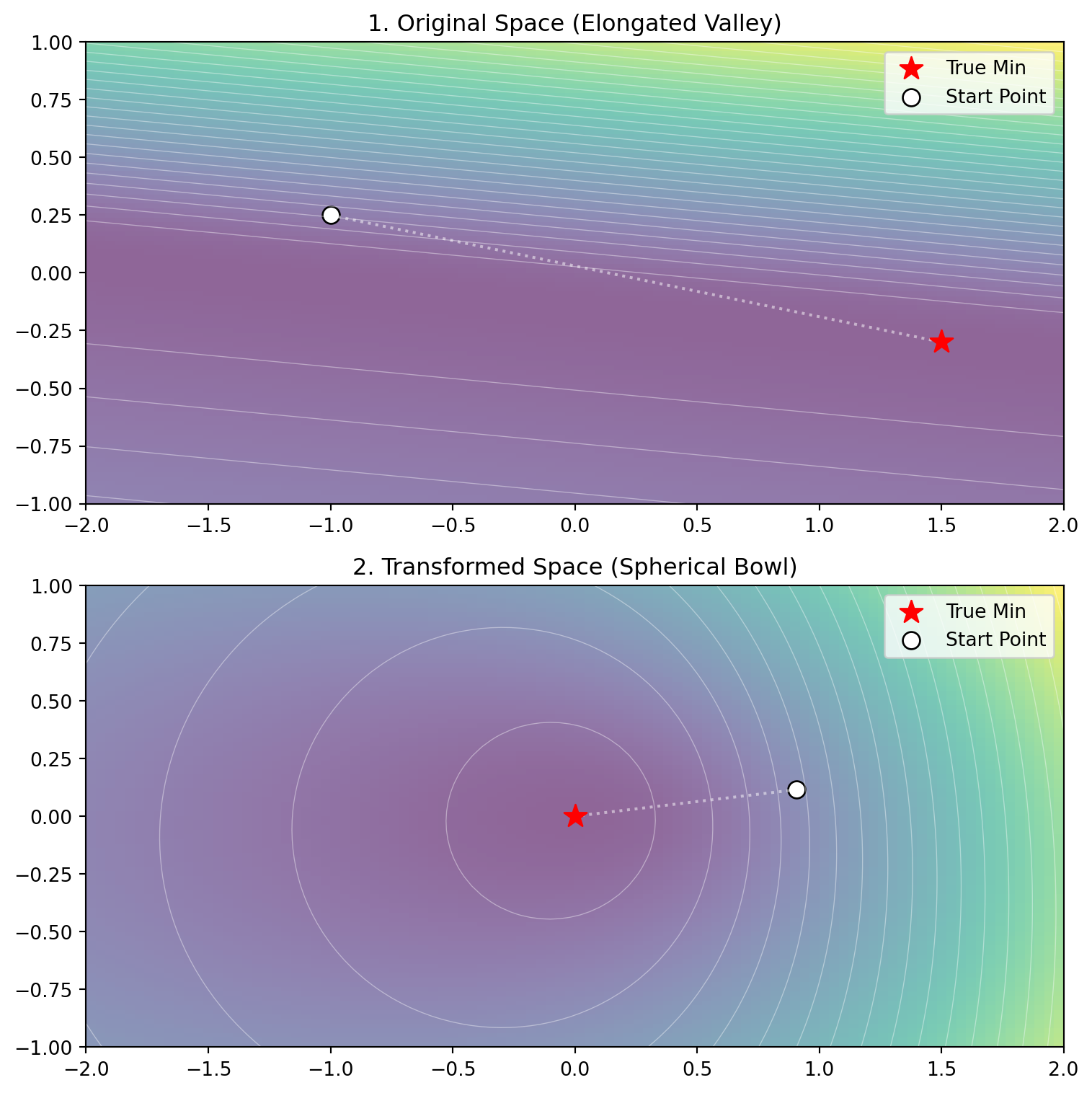
2a. Intuition: Sphering the Landscape
What does multiplying by \mathbf H^{-1} actually do?
Geometrically, the Hessian matrix describes how “distorted” the loss surface is. It tells us that the contours are ellipses, not circles.
The Inverse Hessian acts as a coordinate transformation that undoes this distortion.
It shrinks the directions with high curvature (steep walls).
It stretches the directions with low curvature (flat valley).
Effectively, Newton’s method transforms the “Narrow Valley” back into a perfect, round bowl (“sphering” the data). On a perfect bowl, the gradient points straight at the minimum.
Code
# -----------------------------# Visualization: The "Sphering" Effect# -----------------------------import numpy as npimport matplotlib.pyplot as pltfrom scipy.stats import truncnorm# Re-setup the Nasty Valley data locally for this cell to be self-containednp.random.seed(42)n =10_000x1 = np.random.normal(0, 1, n)x2 =10.0* x1 + np.random.normal(0, .5, n) X = np.column_stack([x1, x2])w_true = np.array([1.5, -0.3]) logits = X @ w_truep =1/ (1+ np.exp(-logits))y = np.random.binomial(1, p)# Helper functionsdef get_hessian(w): p =1/ (1+ np.exp(-X @ w)) weights = p * (1- p) H = (X.T @ (weights[:, None] * X)) / nreturn H# Grid setupw1_vals = np.linspace(-2, 2, 100) # Shifted to see everythingw2_vals = np.linspace(-1, 1, 100)W1, W2 = np.meshgrid(w1_vals, w2_vals)Z = np.zeros_like(W1)for i inrange(W1.shape[0]):for j inrange(W1.shape[1]): w = np.array([W1[i, j], W2[i, j]]) p_val =1/ (1+ np.exp(-X @ w)) eps =1e-12 Z[i, j] =-np.average(y * np.log(p_val + eps) + (1- y) * np.log(1- p_val + eps))# 1. Hessian at the TRUE MINIMUM (Ideal Geometry)# This defines the "perfect bowl" shape we want to transform intoH_star = get_hessian(w_true)# 2. Compute Transformation Matrixtry: L_mat = np.linalg.cholesky(H_star)except np.linalg.LinAlgError: vals, vecs = np.linalg.eigh(H_star) vals = np.maximum(vals, 1e-4) L_mat = vecs @ np.diag(np.sqrt(vals)) @ vecs.T# 3. Setup Plotsfig, axes = plt.subplots(2, 1, figsize=(8, 8))# --- Plot 1: Original Space ---axes[0].imshow( Z, extent=[-2, 2, -1, 1], origin="lower", aspect="auto", cmap="viridis", alpha=0.6)axes[0].contour(W1, W2, Z, levels=np.linspace(Z.min(), Z.max(), 30), colors='white', alpha=0.4, linewidths=0.5)w_bad = np.array([-1, 0.25]) # A visible bad start pointaxes[0].scatter(w_true[0], w_true[1], c='red', marker='*', s=150, zorder=10, label="True Min")axes[0].scatter(w_bad[0], w_bad[1], c='white', s=80, edgecolors='black', label="Start Point")axes[0].plot([w_bad[0], w_true[0]], [w_bad[1], w_true[1]], 'w:', alpha=0.5) # path lineaxes[0].set_title("1. Original Space (Elongated Valley)")axes[0].set_xlim(-2, 2)axes[0].set_ylim(-1, 1)axes[0].legend(loc="upper right")# --- Plot 2: Transformed Space (u space) ---# Transformation: u = L.T @ (w - w_true)# This centers the plot at the true minimum (0,0) and spheres the bowl around it.# Create grid in U space (centered at 0)u_vals = np.linspace(-2, 2, 100)U1_grid, U2_grid = np.meshgrid(u_vals, u_vals)# Inverse transform U grid back to W space to calculate true loss# u = L.T @ (w - w_true) ==> w = L_inv.T @ u + w_trueL_inv_T = np.linalg.inv(L_mat.T)Z_u = np.zeros_like(U1_grid)for i inrange(U1_grid.shape[0]):for j inrange(U1_grid.shape[1]): u_vec = np.array([U1_grid[i, j], U2_grid[i, j]]) w_vec = L_inv_T @ u_vec + w_true# Calculate standard loss at this corresponding w p_val =1/ (1+ np.exp(-X @ w_vec)) eps =1e-12 Z_u[i, j] =-np.average(y * np.log(p_val + eps) + (1- y) * np.log(1- p_val + eps))axes[1].imshow( Z_u, extent=[-2, 2, -1, 1], origin="lower", aspect="auto", cmap="viridis", alpha=0.6)axes[1].contour(U1_grid, U2_grid, Z_u, levels=20, colors='white', alpha=0.4, linewidths=0.5)# Calculate transformed pointsu_min = np.array([0, 0]) # By definitionu_start = L_mat.T @ (w_bad - w_true)axes[1].scatter(u_min[0], u_min[1], c='red', marker='*', s=150, zorder=10, label="True Min")axes[1].scatter(u_start[0], u_start[1], c='white', s=80, edgecolors='black', label="Start Point")axes[1].plot([u_start[0], u_min[0]], [u_start[1], u_min[1]], 'w:', alpha=0.5)# Draw a perfect circle reference to show how spherical the loss is roughlycircle_theta = np.linspace(0, 2*np.pi, 100)#axes[1].plot(np.cos(circle_theta), np.sin(circle_theta), 'w--', alpha=0.3, label="Perfect Sphere Ref")axes[1].set_title("2. Transformed Space (Spherical Bowl)")axes[1].set_xlim(-2, 2)axes[1].set_ylim(-1, 1)axes[1].legend(loc="upper right")plt.tight_layout()plt.show()
Key Intuition: Newton’s method calculates the step you would take if the loss surface were a perfect circle, then projects that back into the real space.
2b. Momentum and Adaptation
Before we look at the results, let’s explicitly connect Newton’s method to the two biggest ideas in modern deep learning optimization: Momentum and Adaptive Gradients.
Newton’s update rule is: \mathbf{w}_{new} = \mathbf{w} - \eta \mathbf{H}^{-1} \nabla L
This single mathematical operation \mathbf{H}^{-1} is actually doing two distinct things at once:
1. It rotates the update (Momentum-like)
The Hessian contains information about how parameters interact (the off-diagonal terms like \frac{\partial^2 L}{\partial w_1 \partial w_2}). By inverting this, Newton’s method realizes, “If I move in w_1, I should also adjust w_2 to compensate.”
Geometrically, this straightens the path. Instead of zig-zagging independently in w_1 and w_2, it cuts diagonally through the valley.
2. It rescales the axes (Adaptive Gradients)
The Hessian contains information about how steep each specific parameter is (the diagonal terms like \frac{\partial^2 L}{\partial w_1^2}). By dividing by this, Newton’s method realizes, “The slope in w_1 is huge, so I should divide by a big number. The slope in w_2 is tiny, so I should divide by a small number.”
This normalizes the step sizes so we move at the same speed in all directions.
3. GD vs Newton
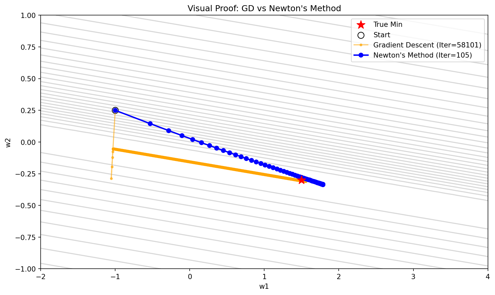
The best way to show the difference between gradient descent and Newton’s method is to show the difference in the path taken from the starting point to the minimum.
Code
# -----------------------------# 1. Setup the Nasty Valley (Exact same problem as Tab 07)# -----------------------------import time np.random.seed(42)n =10_000# x1, x2 generation (ill-conditioned)x1 = np.random.normal(0, 1, n)x2 =10.0* x1 + np.random.normal(0, .5, n) X = np.column_stack([x1, x2])w_true = np.array([1.5, -0.3]) # Labelslogits = X @ w_truep =1/ (1+ np.exp(-logits))y = np.random.binomial(1, p)# Definitionsdef get_loss(w): p =1/ (1+ np.exp(-X @ w)) eps =1e-12return-np.average(y * np.log(p + eps) + (1- y) * np.log(1- p + eps))def get_grad(w): p =1/ (1+ np.exp(-X @ w))return (X.T @ (p - y)) / ndef get_hessian(w): p =1/ (1+ np.exp(-X @ w)) weights = p * (1- p)# H = (1/N) * X.T @ diag(weights) @ Xreturn (X.T @ (weights[:, None] * X)) / n# -----------------------------# 2. Run Comparison# -----------------------------w_start = np.array([-1.0, 0.25]) # Same start as Tab 07tol =1e-4max_iter =100000# --- Standard GD (eta=0.1) ---w = w_start.copy()path_gd = [w.copy()]start_time = time.time()converged_gd =Falsefor i inrange(max_iter): grad = get_grad(w)if np.linalg.norm(grad) < tol: converged_gd =Truebreak w = w -0.1* grad path_gd.append(w.copy())time_gd = time.time() - start_timeiter_gd = i# --- Newton's Method (eta=0.01) ---w = w_start.copy()path_newton = [w.copy()]start_time = time.time()converged_newton =Falsefor i inrange(max_iter): grad = get_grad(w)if np.linalg.norm(grad) < tol: converged_newton =Truebreak H = get_hessian(w)try: step = np.linalg.solve(H, grad)except np.linalg.LinAlgError:break# Use conservative step size for Newton w = w -0.1* step path_newton.append(w.copy())time_newton = time.time() - start_timeiter_newton = ipath_gd = np.array(path_gd)path_newton = np.array(path_newton)# -----------------------------# 3. Plotting# -----------------------------# Recompute Z for backgroundw1_vals = np.linspace(-2, 4, 100)w2_vals = np.linspace(-1, 1, 100)W1, W2 = np.meshgrid(w1_vals, w2_vals)Z = np.zeros_like(W1)for i inrange(W1.shape[0]):for j inrange(W1.shape[1]): Z[i,j] = get_loss(np.array([W1[i,j], W2[i,j]]))plt.figure(figsize=(10, 6))plt.contour(W1, W2, Z, levels=np.logspace(np.log10(Z.min()), np.log10(Z.max()), 30), colors='gray', alpha=0.3)plt.scatter(w_true[0], w_true[1], c='red', marker='*', s=150, zorder=10, label="True Min")plt.scatter(w_start[0], w_start[1], c='white', edgecolors='black', s=80, label="Start")# Plot GDplt.plot(path_gd[:,0], path_gd[:,1], 'o-', label=f"Gradient Descent (Iter={len(path_gd)})", color='orange', markersize=3, alpha=0.6)# Plot Newtonplt.plot(path_newton[:,0], path_newton[:,1], 'o-', label=f"Newton's Method (Iter={len(path_newton)})", color='blue', linewidth=2)plt.title("Visual Proof: GD vs Newton's Method")plt.xlabel("w1")plt.ylabel("w2")plt.legend()plt.tight_layout()plt.show()# -----------------------------# 4. Results Table# -----------------------------from IPython.display import Markdowndef format_res(name, eta, iters, t_sec, w_fin, conv): status ="Converged ✅"if conv else"Slow ⏳" w_s =f"({w_fin[0]:.3f}, {w_fin[1]:.3f})"returnf"| {name} | {eta} | {iters} | {t_sec:.4f} | {w_s} | {status} |"table_md ="""| Method | Step Size | Iterations | Time (s) | Final w | Status ||---|---|---|---|---|---|"""table_md += format_res("Gradient Descent", 0.1, iter_gd, time_gd, path_gd[-1], converged_gd) +"\n"table_md += format_res("Newton's Method", 0.1, iter_newton, time_newton, path_newton[-1], converged_newton) +"\n"Markdown(table_md)
Method
Step Size
Iterations
Time (s)
Final w
Status
Gradient Descent
0.1
58100
2.3771
(1.554, -0.311)
Converged ✅
Newton’s Method
0.1
104
0.0256
(1.786, -0.334)
Converged ✅
Notice exactly what happened:
Gradient Descent flailed around against the steep walls, found the ridge, and slowly descended towards the minimum.
Newton’s Method looked at the curvature, realized the walls were steep, ignored them, and walked almost perfectly straight down the valley floor. It slightly overshoots the minimum, so it traverses back along the same path and then drops onto the minimum. It requires 558x less iterations to complete and 240x less clock time to converge!
Newton’s method effectively “solves” the pathology.
4. The Computational Price Tag
If Newton’s Method is so perfect, why do we need to discuss other optimization methods?
Optimization is “No Free Lunch”. We traded iterations for computation per iteration.
The bottleneck: Inverting H
The Newton step requires solving a system of linear equations involving \mathbf H, a d \times d matrix (where d is the number of parameters).
The computational cost of inverting (or solving) a d \times d matrix scales with O(d^3).
Small NN (d=1,000): 10^9 (1 billion) operations. Doable.
Modern NN (d=1,000,000): 10^{18} (1 quintillion) operations per step. Impossible.
Also, simply storing a Hessian for a 1M parameter model requires 1,000,000 \times 1,000,000 floats, which is roughly 4 Terabytes of RAM.
For high-dimensional problems, this is not possible!
The Strategy for High Dimensional Problems
We are stuck in a dilemma:
Gradient Descent is cheap (O(d)), but dumb (zig-zaggy).
Newton’s Method is smart (straight lines), but prohibitively expensive (O(d^3)).
The entire field of modern optimization involves finding unholy compromises that give us cheap curvature information. We want methods that act like Newton (smart directions) but cost like Gradient Descent (linear scaling).
This motivates the next two major topics:
Momentum: Uses physical velocity to smooth out zig-zags without calculating curvature.
Adaptive Methods (RMSProp, Adam): Uses the history of gradients to approximate the diagonal of the Hessian, effectively creating a “poor man’s Newton’s method.”
Source Code
---title: "08: Newton's Method"format: html: code-fold: truejupyter: python3---## The solution to "Pathologies"In the previous section, we saw that standard Gradient Descent fails when the loss landscape is "ill-conditioned"—shaped like a narrow taco or a long canyon.This happens because GD is **isotropic**: it treats every direction in parameter space the same.- It sees a steep slope (the canyon walls) and thinks "I should take a big step this way."- It sees a flat slope (the valley floor) and thinks "I should take a tiny step this way."This is exactly the **opposite** of what we want. We want to move *cautiously* in steep directions and *aggressively* in flat directions.**Newton's Method** solves this by using **curvature** information (second derivatives) to measure the shape of the landscape and correct the step size for every direction individually.---## 1. The Geometry of CurvatureWe previously defined the Gradient $\nabla L$ (slope). Now we stick with the Hessian $\mathbf H$ (curvature).For a function with two parameters $w_1, w_2$, the Hessian is the $2 \times 2$ matrix of second derivatives:$$\mathbf H(\mathbf w) = \begin{bmatrix}\frac{\partial^2 L}{\partial w_1^2} & \frac{\partial^2 L}{\partial w_1 \partial w_2} \\\frac{\partial^2 L}{\partial w_2 \partial w_1} & \frac{\partial^2 L}{\partial w_2^2}\end{bmatrix}$$### The Taylor ApproximationGradient Descent approximates the loss as a **plane** (linear).Newton's Method approximates the loss as a **bowl** (quadratic).$$L(\mathbf w + \Delta) \approx L(\mathbf w) + \nabla L^\top \Delta + \frac{1}{2}\Delta^\top \mathbf H \Delta$$If we find the $\Delta$ that minimizes this quadratic approximation (by setting the derivative to zero), we get the Newton update rule:$$\mathbf w_{new} = \mathbf w_{old} - \eta \underbrace{\mathbf H^{-1} \nabla L}_{\text{Newton Step}}$$Compare this to Gradient Descent:1. **GD**: $\mathbf w_{new} = \mathbf w - \eta \nabla L$2. **Newton**: $\mathbf w_{new} = \mathbf w - \eta \mathbf H^{-1} \nabla L$The difference is the **Inverse Hessian** $\mathbf H^{-1}$.**Note:** While Newton updates do not require a step size (e.g. $\eta = 1$), it is often advised to introduce one to dampen the Newton updates at the original "bad" starting points.---## 2a. Intuition: Sphering the LandscapeWhat does multiplying by $\mathbf H^{-1}$ actually *do*?Geometrically, the Hessian matrix describes how "distorted" the loss surface is. It tells us that the contours are ellipses, not circles.The **Inverse Hessian** acts as a coordinate transformation that **undoes this distortion**.1. It shrinks the directions with high curvature (steep walls).2. It stretches the directions with low curvature (flat valley).Effectively, Newton's method transforms the "Narrow Valley" back into a perfect, round bowl ("sphering" the data). On a perfect bowl, the gradient points straight at the minimum.```{python}# -----------------------------# Visualization: The "Sphering" Effect# -----------------------------import numpy as npimport matplotlib.pyplot as pltfrom scipy.stats import truncnorm# Re-setup the Nasty Valley data locally for this cell to be self-containednp.random.seed(42)n =10_000x1 = np.random.normal(0, 1, n)x2 =10.0* x1 + np.random.normal(0, .5, n) X = np.column_stack([x1, x2])w_true = np.array([1.5, -0.3]) logits = X @ w_truep =1/ (1+ np.exp(-logits))y = np.random.binomial(1, p)# Helper functionsdef get_hessian(w): p =1/ (1+ np.exp(-X @ w)) weights = p * (1- p) H = (X.T @ (weights[:, None] * X)) / nreturn H# Grid setupw1_vals = np.linspace(-2, 2, 100) # Shifted to see everythingw2_vals = np.linspace(-1, 1, 100)W1, W2 = np.meshgrid(w1_vals, w2_vals)Z = np.zeros_like(W1)for i inrange(W1.shape[0]):for j inrange(W1.shape[1]): w = np.array([W1[i, j], W2[i, j]]) p_val =1/ (1+ np.exp(-X @ w)) eps =1e-12 Z[i, j] =-np.average(y * np.log(p_val + eps) + (1- y) * np.log(1- p_val + eps))# 1. Hessian at the TRUE MINIMUM (Ideal Geometry)# This defines the "perfect bowl" shape we want to transform intoH_star = get_hessian(w_true)# 2. Compute Transformation Matrixtry: L_mat = np.linalg.cholesky(H_star)except np.linalg.LinAlgError: vals, vecs = np.linalg.eigh(H_star) vals = np.maximum(vals, 1e-4) L_mat = vecs @ np.diag(np.sqrt(vals)) @ vecs.T# 3. Setup Plotsfig, axes = plt.subplots(2, 1, figsize=(8, 8))# --- Plot 1: Original Space ---axes[0].imshow( Z, extent=[-2, 2, -1, 1], origin="lower", aspect="auto", cmap="viridis", alpha=0.6)axes[0].contour(W1, W2, Z, levels=np.linspace(Z.min(), Z.max(), 30), colors='white', alpha=0.4, linewidths=0.5)w_bad = np.array([-1, 0.25]) # A visible bad start pointaxes[0].scatter(w_true[0], w_true[1], c='red', marker='*', s=150, zorder=10, label="True Min")axes[0].scatter(w_bad[0], w_bad[1], c='white', s=80, edgecolors='black', label="Start Point")axes[0].plot([w_bad[0], w_true[0]], [w_bad[1], w_true[1]], 'w:', alpha=0.5) # path lineaxes[0].set_title("1. Original Space (Elongated Valley)")axes[0].set_xlim(-2, 2)axes[0].set_ylim(-1, 1)axes[0].legend(loc="upper right")# --- Plot 2: Transformed Space (u space) ---# Transformation: u = L.T @ (w - w_true)# This centers the plot at the true minimum (0,0) and spheres the bowl around it.# Create grid in U space (centered at 0)u_vals = np.linspace(-2, 2, 100)U1_grid, U2_grid = np.meshgrid(u_vals, u_vals)# Inverse transform U grid back to W space to calculate true loss# u = L.T @ (w - w_true) ==> w = L_inv.T @ u + w_trueL_inv_T = np.linalg.inv(L_mat.T)Z_u = np.zeros_like(U1_grid)for i inrange(U1_grid.shape[0]):for j inrange(U1_grid.shape[1]): u_vec = np.array([U1_grid[i, j], U2_grid[i, j]]) w_vec = L_inv_T @ u_vec + w_true# Calculate standard loss at this corresponding w p_val =1/ (1+ np.exp(-X @ w_vec)) eps =1e-12 Z_u[i, j] =-np.average(y * np.log(p_val + eps) + (1- y) * np.log(1- p_val + eps))axes[1].imshow( Z_u, extent=[-2, 2, -1, 1], origin="lower", aspect="auto", cmap="viridis", alpha=0.6)axes[1].contour(U1_grid, U2_grid, Z_u, levels=20, colors='white', alpha=0.4, linewidths=0.5)# Calculate transformed pointsu_min = np.array([0, 0]) # By definitionu_start = L_mat.T @ (w_bad - w_true)axes[1].scatter(u_min[0], u_min[1], c='red', marker='*', s=150, zorder=10, label="True Min")axes[1].scatter(u_start[0], u_start[1], c='white', s=80, edgecolors='black', label="Start Point")axes[1].plot([u_start[0], u_min[0]], [u_start[1], u_min[1]], 'w:', alpha=0.5)# Draw a perfect circle reference to show how spherical the loss is roughlycircle_theta = np.linspace(0, 2*np.pi, 100)#axes[1].plot(np.cos(circle_theta), np.sin(circle_theta), 'w--', alpha=0.3, label="Perfect Sphere Ref")axes[1].set_title("2. Transformed Space (Spherical Bowl)")axes[1].set_xlim(-2, 2)axes[1].set_ylim(-1, 1)axes[1].legend(loc="upper right")plt.tight_layout()plt.show()```> **Key Intuition**: Newton's method calculates the step you *would* take if the loss surface were a perfect circle, then projects that back into the real space.---## 2b. Momentum and AdaptationBefore we look at the results, let's explicitly connect Newton's method to the two biggest ideas in modern deep learning optimization: **Momentum** and **Adaptive Gradients**.Newton's update rule is:$$ \mathbf{w}_{new} = \mathbf{w} - \eta \mathbf{H}^{-1} \nabla L $$This single mathematical operation $\mathbf{H}^{-1}$ is actually doing **two** distinct things at once:### 1. It rotates the update (Momentum-like)The Hessian contains information about how parameters interact (the off-diagonal terms like $\frac{\partial^2 L}{\partial w_1 \partial w_2}$).By inverting this, Newton's method realizes, *"If I move in $w_1$, I should also adjust $w_2$ to compensate."*Geometrically, this straightens the path. Instead of zig-zagging independently in $w_1$ and $w_2$, it cuts diagonally through the valley.### 2. It rescales the axes (Adaptive Gradients)The Hessian contains information about how steep each specific parameter is (the diagonal terms like $\frac{\partial^2 L}{\partial w_1^2}$).By dividing by this, Newton's method realizes, *"The slope in $w_1$ is huge, so I should divide by a big number. The slope in $w_2$ is tiny, so I should divide by a small number."*This normalizes the step sizes so we move at the same speed in all directions.---## 3. GD vs NewtonThe best way to show the difference between gradient descent and Newton's method is to show the difference in the path taken from the starting point to the minimum.```{python}# -----------------------------# 1. Setup the Nasty Valley (Exact same problem as Tab 07)# -----------------------------import time np.random.seed(42)n =10_000# x1, x2 generation (ill-conditioned)x1 = np.random.normal(0, 1, n)x2 =10.0* x1 + np.random.normal(0, .5, n) X = np.column_stack([x1, x2])w_true = np.array([1.5, -0.3]) # Labelslogits = X @ w_truep =1/ (1+ np.exp(-logits))y = np.random.binomial(1, p)# Definitionsdef get_loss(w): p =1/ (1+ np.exp(-X @ w)) eps =1e-12return-np.average(y * np.log(p + eps) + (1- y) * np.log(1- p + eps))def get_grad(w): p =1/ (1+ np.exp(-X @ w))return (X.T @ (p - y)) / ndef get_hessian(w): p =1/ (1+ np.exp(-X @ w)) weights = p * (1- p)# H = (1/N) * X.T @ diag(weights) @ Xreturn (X.T @ (weights[:, None] * X)) / n# -----------------------------# 2. Run Comparison# -----------------------------w_start = np.array([-1.0, 0.25]) # Same start as Tab 07tol =1e-4max_iter =100000# --- Standard GD (eta=0.1) ---w = w_start.copy()path_gd = [w.copy()]start_time = time.time()converged_gd =Falsefor i inrange(max_iter): grad = get_grad(w)if np.linalg.norm(grad) < tol: converged_gd =Truebreak w = w -0.1* grad path_gd.append(w.copy())time_gd = time.time() - start_timeiter_gd = i# --- Newton's Method (eta=0.01) ---w = w_start.copy()path_newton = [w.copy()]start_time = time.time()converged_newton =Falsefor i inrange(max_iter): grad = get_grad(w)if np.linalg.norm(grad) < tol: converged_newton =Truebreak H = get_hessian(w)try: step = np.linalg.solve(H, grad)except np.linalg.LinAlgError:break# Use conservative step size for Newton w = w -0.1* step path_newton.append(w.copy())time_newton = time.time() - start_timeiter_newton = ipath_gd = np.array(path_gd)path_newton = np.array(path_newton)# -----------------------------# 3. Plotting# -----------------------------# Recompute Z for backgroundw1_vals = np.linspace(-2, 4, 100)w2_vals = np.linspace(-1, 1, 100)W1, W2 = np.meshgrid(w1_vals, w2_vals)Z = np.zeros_like(W1)for i inrange(W1.shape[0]):for j inrange(W1.shape[1]): Z[i,j] = get_loss(np.array([W1[i,j], W2[i,j]]))plt.figure(figsize=(10, 6))plt.contour(W1, W2, Z, levels=np.logspace(np.log10(Z.min()), np.log10(Z.max()), 30), colors='gray', alpha=0.3)plt.scatter(w_true[0], w_true[1], c='red', marker='*', s=150, zorder=10, label="True Min")plt.scatter(w_start[0], w_start[1], c='white', edgecolors='black', s=80, label="Start")# Plot GDplt.plot(path_gd[:,0], path_gd[:,1], 'o-', label=f"Gradient Descent (Iter={len(path_gd)})", color='orange', markersize=3, alpha=0.6)# Plot Newtonplt.plot(path_newton[:,0], path_newton[:,1], 'o-', label=f"Newton's Method (Iter={len(path_newton)})", color='blue', linewidth=2)plt.title("Visual Proof: GD vs Newton's Method")plt.xlabel("w1")plt.ylabel("w2")plt.legend()plt.tight_layout()plt.show()# -----------------------------# 4. Results Table# -----------------------------from IPython.display import Markdowndef format_res(name, eta, iters, t_sec, w_fin, conv): status ="Converged ✅"if conv else"Slow ⏳" w_s =f"({w_fin[0]:.3f}, {w_fin[1]:.3f})"returnf"| {name} | {eta} | {iters} | {t_sec:.4f} | {w_s} | {status} |"table_md ="""| Method | Step Size | Iterations | Time (s) | Final w | Status ||---|---|---|---|---|---|"""table_md += format_res("Gradient Descent", 0.1, iter_gd, time_gd, path_gd[-1], converged_gd) +"\n"table_md += format_res("Newton's Method", 0.1, iter_newton, time_newton, path_newton[-1], converged_newton) +"\n"Markdown(table_md)```Notice exactly what happened:- **Gradient Descent** flailed around against the steep walls, found the ridge, and slowly descended towards the minimum.- **Newton's Method** looked at the curvature, realized the walls were steep, ignored them, and walked almost perfectly straight down the valley floor. It slightly overshoots the minimum, so it traverses back along the same path and then drops onto the minimum. It requires 558x less iterations to complete and 240x less clock time to converge! Newton's method effectively "solves" the pathology.---## 4. The Computational Price TagIf Newton's Method is so perfect, why do we need to discuss other optimization methods?Optimization is "No Free Lunch". We traded **iterations** for **computation per iteration**.### The bottleneck: Inverting HThe Newton step requires solving a system of linear equations involving $\mathbf H$, a $d \times d$ matrix (where $d$ is the number of parameters).The computational cost of inverting (or solving) a $d \times d$ matrix scales with **$O(d^3)$**.* **Logistic Regression** ($d=2$): $2^3 = 8$ operations. Trivial.* **Small NN** ($d=1,000$): $10^9$ (1 billion) operations. Doable.* **Modern NN** ($d=1,000,000$): $10^{18}$ (1 quintillion) operations per step. **Impossible.**Also, simply *storing* a Hessian for a 1M parameter model requires 1,000,000 $\times$ 1,000,000 floats, which is roughly **4 Terabytes of RAM**.For high-dimensional problems, this is not possible!### The Strategy for High Dimensional ProblemsWe are stuck in a dilemma:1. **Gradient Descent** is cheap ($O(d)$), but dumb (zig-zaggy).2. **Newton's Method** is smart (straight lines), but prohibitively expensive ($O(d^3)$).The entire field of modern optimization involves finding unholy compromises that give us **cheap curvature information**. We want methods that act *like* Newton (smart directions) but cost *like* Gradient Descent (linear scaling).This motivates the next two major topics:1. **Momentum**: Uses physical velocity to smooth out zig-zags without calculating curvature.2. **Adaptive Methods (RMSProp, Adam)**: Uses the history of gradients to *approximate* the diagonal of the Hessian, effectively creating a "poor man's Newton's method."