07: Step Size & Pathologies

Why this matters

Gradient descent is conceptually simple—but its performance lives or dies by the step size.

A bad step size can cause: - divergence, - violent oscillation, - or painfully slow convergence.

Even when the loss is convex (as in logistic regression), optimization can still be hard because the geometry of the loss surface may be highly unfavorable.

In modern deep learning, we do not choose step sizes analytically.
Instead, we rely on empirical diagnostics and learning-rate schedules.

This section explains why that is necessary.

---

Step size matters

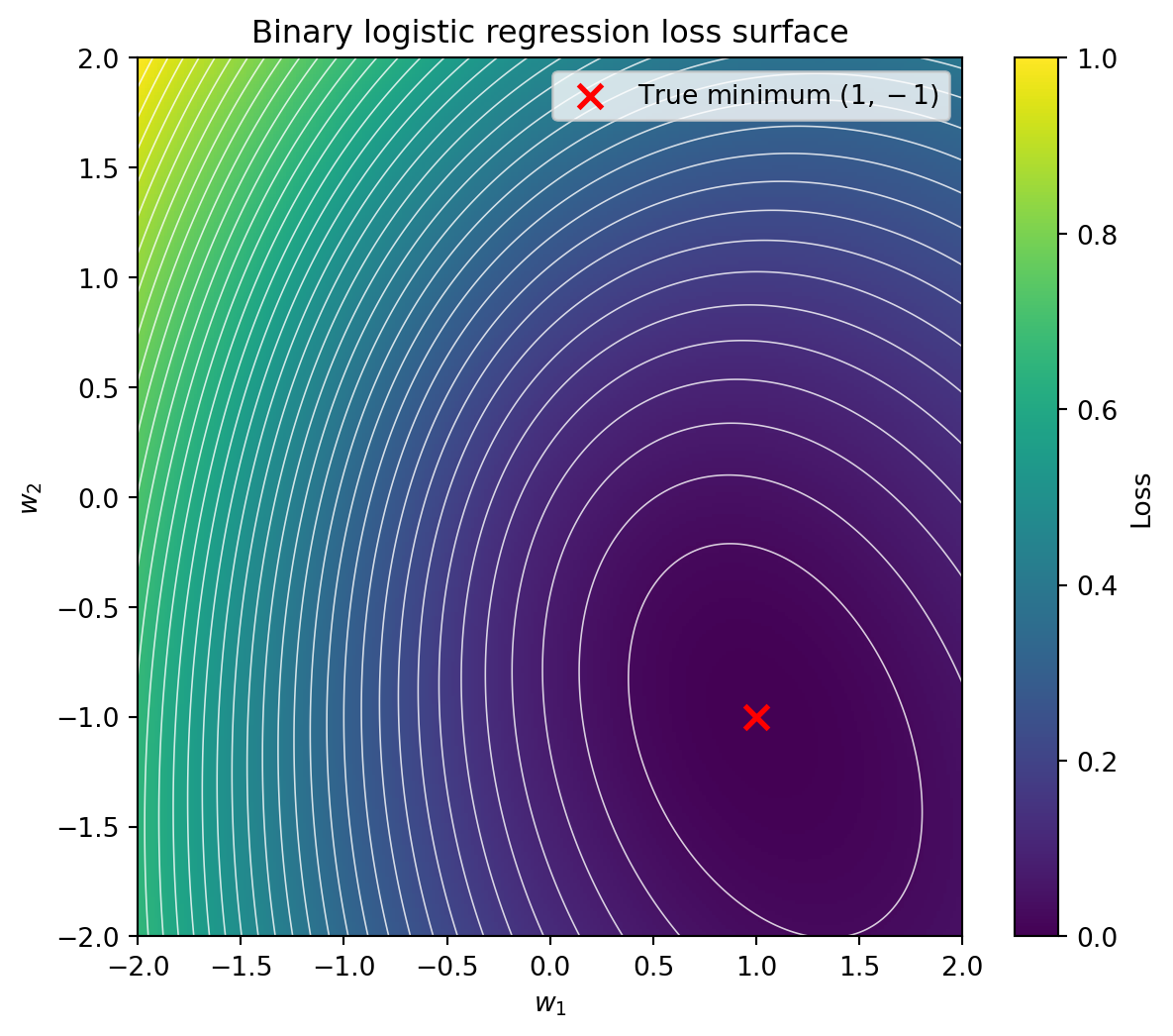
Gradient descent is only guaranteed to work when \eta = \epsilon. Unfortunately, setting the learning rate to the machine minimum (something like 1 \times 10^{-8}) would cause the iterative procedure to take an eternity to finish. Instead, practical GD implementations choose a small step size that cuts the difference between time and stability. To see this, let’s look back at our previous logistic regression problem:

Code

import numpy as np
import matplotlib.pyplot as plt
from scipy.stats import truncnorm

# -----------------------------
# Data generation
# -----------------------------
np.random.seed(42)
n = 10_000

# x1 ~ Uniform(-2, 2)
x1 = np.random.uniform(-2, 2, n)

# x2 correlated with x1 (~0.5)
eps = np.random.normal(0, 1, n)
x2_raw = 0.5 * x1 + np.sqrt(1 - 0.5**2) * eps

# Truncate x2 to [-2, 2]
a, b = (-2 - np.mean(x2_raw)) / np.std(x2_raw), (2 - np.mean(x2_raw)) / np.std(x2_raw)
x2 = truncnorm.rvs(a, b, loc=np.mean(x2_raw), scale=np.std(x2_raw), size=n)

X = np.column_stack([x1, x2])

# True parameters
w_true = np.array([1.0, -1.0])

# Generate labels
logits = X @ w_true
p = 1 / (1 + np.exp(-logits))
y = np.random.binomial(1, p)

def logistic_loss(w, X, y):
    z = X @ w
    p = 1 / (1 + np.exp(-z))
    eps = 1e-12  # numerical safety
    return -np.average(y * np.log(p + eps) + (1 - y) * np.log(1 - p + eps))
  
# Grid for parameters
w1_vals = np.linspace(-2, 2, 250)
w2_vals = np.linspace(-2, 2, 250)

W1, W2 = np.meshgrid(w1_vals, w2_vals)
Z = np.zeros_like(W1)

for i in range(W1.shape[0]):
    for j in range(W1.shape[1]):
        w = np.array([W1[i, j], W2[i, j]])
        Z[i, j] = logistic_loss(w, X, y)
        
plt.figure(figsize=(7, 6))

# Heatmap
plt.imshow(
    Z,
    extent=[-2, 2, -2, 2],
    origin="lower",
    aspect="auto",
    cmap="viridis"
)

# Contour lines (this is the key R-like part)
contour_levels = np.linspace(Z.min(), Z.max(), 40)
plt.contour(
    W1,
    W2,
    Z,
    levels=contour_levels,
    colors="white",
    linewidths=0.6,
    alpha=0.8
)

# Mark true minimum
plt.scatter(
    w_true[0],
    w_true[1],
    color="red",
    s=80,
    marker="x",
    linewidths=2,
    label="True minimum $(1,-1)$"
)

plt.colorbar(label="Loss")
plt.xlabel("$w_1$")
plt.ylabel("$w_2$")
plt.title("Binary logistic regression loss surface")
plt.legend()
plt.show()

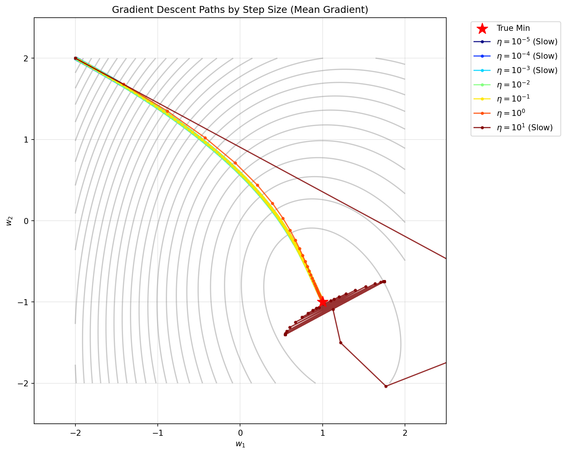
Starting at (-2,2), let’s see how the performance of gradient descent changes as the step size changes. Note that we terminate the gradient descent routine if the norm of the gradient is less than 10^{-4} or we reach 10,000 iterations:

Code

# -----------------------------
# Gradient Descent with Multiple Learning Rates
# -----------------------------
import time

# Define gradient function (Mean Gradient)
def logistic_grad(w, X, y):
    z = X @ w
    p = 1 / (1 + np.exp(-z))
    # Divide by N to get the average gradient
    return (X.T @ (p - y)) / X.shape[0]

# Settings
w_start = np.array([-2.0, 2.0])
learning_rates = [10**i for i in range(-5, 2)] # 1e-5 to 10
max_iter = 10000
tol = 1e-4

results = []
paths = {}

for eta in learning_rates:
    w = w_start.copy()
    path = [w.copy()]
    converged = False
    diverged = False
    
    start_time = time.time()
    
    for t in range(max_iter):
        grad = logistic_grad(w, X, y)
        grad_norm = np.linalg.norm(grad)
        
        # Check stopping condition (Gradient Norm)
        if grad_norm < tol:
            converged = True
            break
            
        # Update weights
        w = w - eta * grad
        path.append(w.copy())
        
        # Safety break for divergence
        if np.linalg.norm(w) > 100:
            diverged = True
            break
            
    end_time = time.time()
    elapsed = end_time - start_time
            
    paths[eta] = np.array(path)
    results.append({
        "eta": eta,
        "iters": t + 1 if t < max_iter - 1 else max_iter,
        "final_w": w,
        "converged": converged,
        "diverged": diverged,
        "time": elapsed
    })

# -----------------------------
# Plotting
# -----------------------------
plt.figure(figsize=(10, 8))

# Background contours
plt.contour(W1, W2, Z, levels=np.linspace(Z.min(), Z.max(), 30), colors='gray', alpha=0.4)
plt.scatter(w_true[0], w_true[1], c='red', marker='*', s=200, label='True Min', zorder=10)

# Plot paths
colors = plt.cm.jet(np.linspace(0, 1, len(learning_rates)))

for i, eta in enumerate(learning_rates):
    path = paths[eta]
    
    # Label handling
    status = ""
    if results[i]['diverged']: status = " (Diverged)"
    elif not results[i]['converged']: status = " (Slow)"
    
    label = f"$\eta = 10^{{{int(np.log10(eta))}}}${status}"
    
    # Only plot if not immediately diverged to infinity
    if len(path) > 1:
        plt.plot(path[:, 0], path[:, 1], 'o-', markersize=3, label=label, color=colors[i], alpha=0.8)

plt.xlim(-2.5, 2.5)
plt.ylim(-2.5, 2.5)
plt.xlabel("$w_1$")
plt.ylabel("$w_2$")
plt.title("Gradient Descent Paths by Step Size (Mean Gradient)")
plt.legend(bbox_to_anchor=(1.05, 1), loc='upper left')
plt.grid(True, alpha=0.3)
plt.tight_layout()
plt.show()

# -----------------------------
# Results Table
# -----------------------------
from IPython.display import Markdown

table_md = "| Learning Rate | Iterations | Time (s) | Final w | Status |\n|---|---|---|---|---|\n"

for res in results:
    eta_str = f"10^{{{int(np.log10(res['eta']))}}}"
    w_str = f"({res['final_w'][0]:.3f}, {res['final_w'][1]:.3f})"
    time_str = f"{res['time']:.4f}"
    
    if res['diverged']:
        status = "Diverged 💥"
    elif res['converged']:
        status = "Converged ✅"
    else:
        status = "Did not converge ⏳"
        
    table_md += f"| ${eta_str}$ | {res['iters']} | {time_str} | {w_str} | {status} |\n"

Markdown(table_md)

Learning Rate	Iterations	Time (s)	Final w	Status
10^{-5}	10000	0.3535	(-1.942, 1.968)	Did not converge ⏳
10^{-4}	10000	0.3528	(-1.438, 1.675)	Did not converge ⏳
10^{-3}	10000	0.4028	(0.657, -0.280)	Did not converge ⏳
10^{-2}	7685	0.2740	(1.017, -1.024)	Converged ✅
10^{-1}	766	0.0278	(1.017, -1.024)	Converged ✅
10^{0}	74	0.0026	(1.017, -1.024)	Converged ✅
10^{1}	10000	0.3773	(1.747, -0.747)	Did not converge ⏳

Here we can see the step size problem:

• Too small of learning rate means that we never get to the minimum from our starting point. This costs us time.
• Learning rates in the correct magnitude range get to the minimum before the maximum number of iterations is reached. However, the “right” learning rate gets us there 235 times faster than a suboptimal learning rate.
• Too big of a learning rate shoots off the loss surface to start and then slowly approaches the minimum. Once it gets around the minimum it oscillates uncontrollably meaning that we never converge. This costs us both time and accuracy!

Step size matters even more for ill conditioned problems!

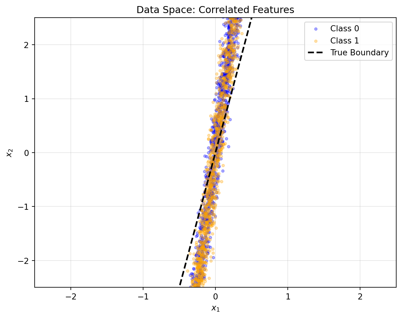
With relatively low correlation between features, logistic regression is a quite well behaved problem. Now, let’s create a realistic scenario where things aren’t as nice.

Code

import numpy as np
import matplotlib.pyplot as plt
from scipy.stats import truncnorm

# -----------------------------
# Data generation: The "Narrow Valley" Pathology
# -----------------------------
np.random.seed(42)
n = 10_000

# 1. Create highly correlated features
# x1 is small scale
x1 = np.random.normal(0, 1, n)

# x2 is highly correlated with x1 but on a MUCH larger scale
# This creates the "narrow valley" effect where w2 changes affect loss 
# much more drastically than w1 changes.
x2 = 10.0 * x1 + np.random.normal(0, .5, n) 

X = np.column_stack([x1, x2])

# True parameters (The valley floor)
w_true = np.array([1.5, -0.3]) 

# Generate labels
logits = X @ w_true
p = 1 / (1 + np.exp(-logits))
y = np.random.binomial(1, p)

# -----------------------------
# Plot 1: Data Space
# -----------------------------
plt.figure(figsize=(8, 6))

# Scatter plot of x1 vs x2 colored by class
plt.scatter(X[y==0, 0], X[y==0, 1], alpha=0.3, s=10, label='Class 0', c='blue')
plt.scatter(X[y==1, 0], X[y==1, 1], alpha=0.3, s=10, label='Class 1', c='orange')

# Draw the true decision boundary: w1*x1 + w2*x2 = 0 => x2 = -(w1/w2)*x1
x_line = np.linspace(-2, 2, 100)
y_line = -(w_true[0] / w_true[1]) * x_line
plt.plot(x_line, y_line, 'k--', linewidth=2, label='True Boundary')

plt.xlim(-2.5, 2.5)
plt.ylim(-2.5, 2.5)
plt.xlabel("$x_1$")
plt.ylabel("$x_2$")
plt.title("Data Space: Correlated Features")
plt.legend()
plt.grid(True, alpha=0.3)
plt.show()

Code

# -----------------------------
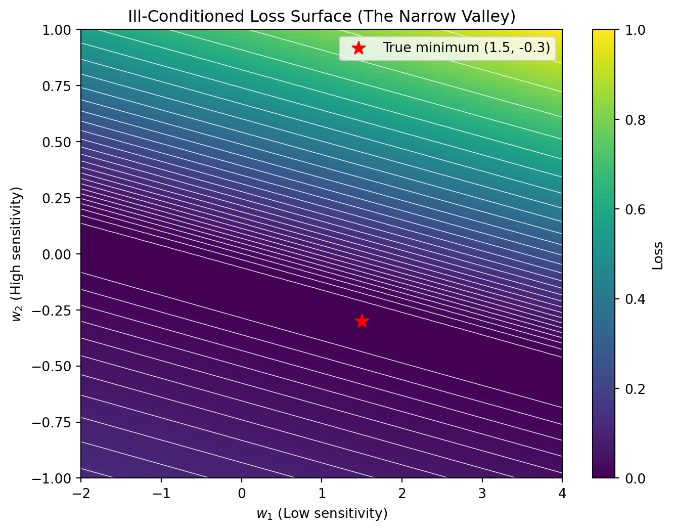
# Plot 2: Loss Surface
# -----------------------------
def logistic_loss(w, X, y):
    z = X @ w
    p = 1 / (1 + np.exp(-z))
    eps = 1e-12
    return -np.average(y * np.log(p + eps) + (1 - y) * np.log(1 - p + eps))
  
# Grid for parameters - Zoomed out to see the valley
w1_vals = np.linspace(-2, 4, 100)
w2_vals = np.linspace(-1, 1, 100)

W1, W2 = np.meshgrid(w1_vals, w2_vals)
Z = np.zeros_like(W1)

for i in range(W1.shape[0]):
    for j in range(W1.shape[1]):
        w = np.array([W1[i, j], W2[i, j]])
        Z[i, j] = logistic_loss(w, X, y)
        
plt.figure(figsize=(8, 6))

# Heatmap
plt.imshow(
    Z,
    extent=[-2, 4, -1, 1],
    origin="lower",
    aspect="auto",
    cmap="viridis"
)

# Contour lines - Use log spacing to see details in the valley
contour_levels = np.logspace(np.log10(Z.min()), np.log10(Z.max()), 30)
plt.contour(
    W1,
    W2,
    Z,
    levels=contour_levels,
    colors="white",
    linewidths=0.6,
    alpha=0.8
)

# Mark true minimum
plt.scatter(
    w_true[0],
    w_true[1],
    color="red",
    s=100,
    marker="*",
    label=f"True minimum ({w_true[0]}, {w_true[1]})"
)

plt.colorbar(label="Loss")
plt.xlabel("$w_1$ (Low sensitivity)")
plt.ylabel("$w_2$ (High sensitivity)")
plt.title("Ill-Conditioned Loss Surface (The Narrow Valley)")
plt.legend()
plt.show()

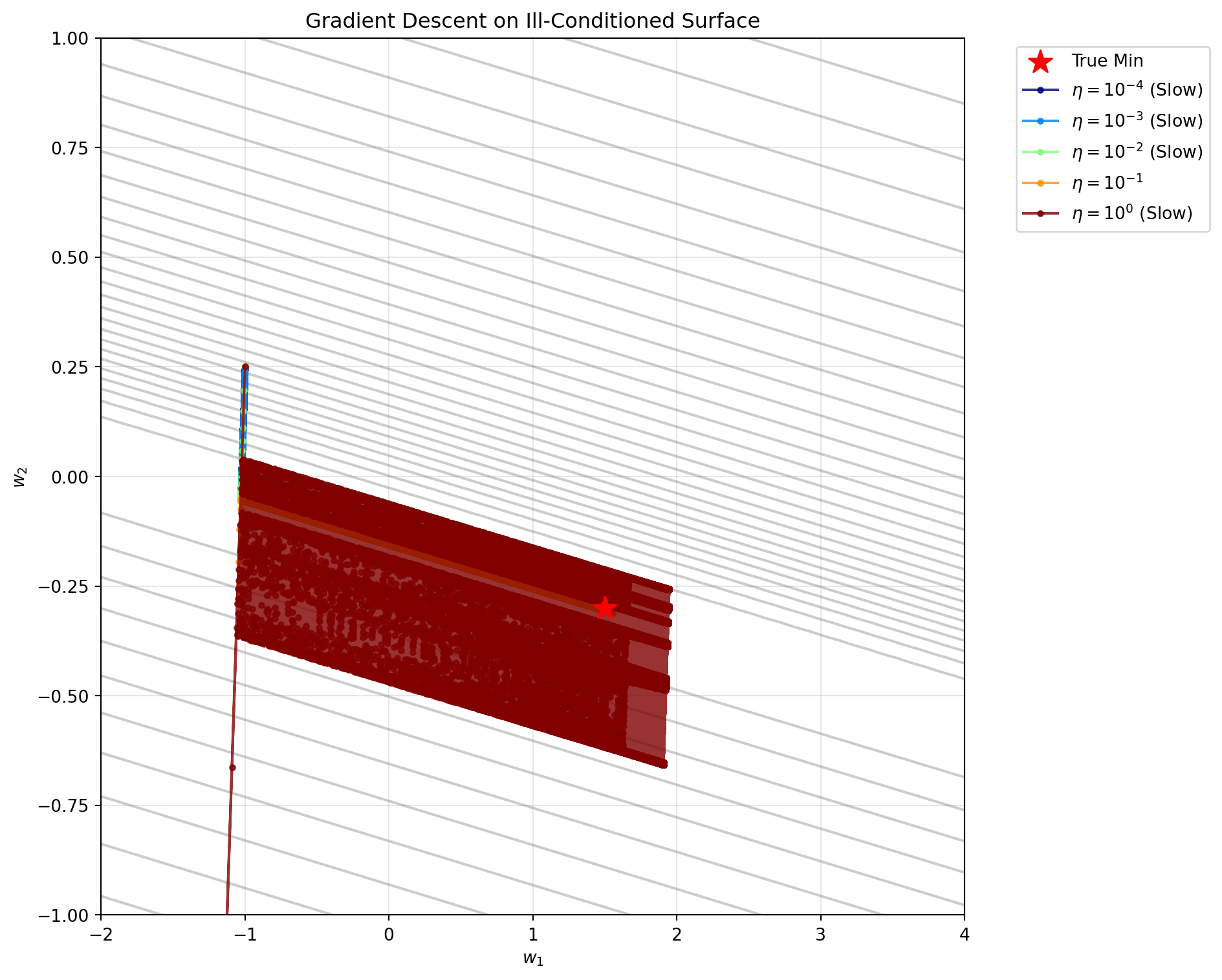
Here, we have an example with a long and narrow valley. Let’s see how our gradient descent routine works here:

Code

# -----------------------------
# Gradient Descent with Multiple Learning Rates
# -----------------------------
import time

# Define gradient function (Mean Gradient)
def logistic_grad(w, X, y):
    z = X @ w
    p = 1 / (1 + np.exp(-z))
    return (X.T @ (p - y)) / X.shape[0]

# Settings
# Start far away to force it to traverse the valley
w_start = np.array([-1, .25]) 
learning_rates = [10**i for i in range(-4, 0)] + [10**-.5] # Adjusted range for this problem
max_iter = 100000
tol = 1e-4

results = []
paths = {}

for eta in learning_rates:
    w = w_start.copy()
    path = [w.copy()]
    converged = False
    diverged = False
    
    start_time = time.time()
    
    for t in range(max_iter):
        grad = logistic_grad(w, X, y)
        grad_norm = np.linalg.norm(grad)
        
        if grad_norm < tol:
            converged = True
            break
            
        w = w - eta * grad
        path.append(w.copy())
        
        if np.linalg.norm(w) > 100:
            diverged = True
            break
            
    end_time = time.time()
    elapsed = end_time - start_time
            
    paths[eta] = np.array(path)
    results.append({
        "eta": eta,
        "iters": t + 1 if t < max_iter - 1 else max_iter,
        "final_w": w,
        "converged": converged,
        "diverged": diverged,
        "time": elapsed
    })

# -----------------------------
# Plotting
# -----------------------------
plt.figure(figsize=(10, 8))

# Background contours
plt.contour(W1, W2, Z, levels=np.logspace(np.log10(Z.min()), np.log10(Z.max()), 30), colors='gray', alpha=0.4)
plt.scatter(w_true[0], w_true[1], c='red', marker='*', s=200, label='True Min', zorder=10)

# Plot paths
colors = plt.cm.jet(np.linspace(0, 1, len(learning_rates)))

for i, eta in enumerate(learning_rates):
    path = paths[eta]
    
    status = ""
    if results[i]['diverged']: status = " (Diverged)"
    elif not results[i]['converged']: status = " (Slow)"
    
    label = f"$\eta = 10^{{{int(np.log10(eta))}}}${status}"
    
    if len(path) > 1:
        plt.plot(path[:, 0], path[:, 1], 'o-', markersize=3, label=label, color=colors[i], alpha=0.8)

plt.xlim(-2, 4)
plt.ylim(-1, 1)
plt.xlabel("$w_1$")
plt.ylabel("$w_2$")
plt.title("Gradient Descent on Ill-Conditioned Surface")
plt.legend(bbox_to_anchor=(1.05, 1), loc='upper left')
plt.grid(True, alpha=0.3)
plt.tight_layout()
plt.show()

# -----------------------------
# Results Table
# -----------------------------
from IPython.display import Markdown

table_md = "| Learning Rate | Iterations | Time (s) | Final w | Status |\n|---|---|---|---|---|\n"

for res in results:
    eta_str = f"10^{{{int(np.log10(res['eta']))}}}"
    w_str = f"({res['final_w'][0]:.3f}, {res['final_w'][1]:.3f})"
    time_str = f"{res['time']:.4f}"
    
    if res['diverged']:
        status = "Diverged 💥"
    elif res['converged']:
        status = "Converged ✅"
    else:
        status = "Did not converge ⏳"
        
    table_md += f"| ${eta_str}$ | {res['iters']} | {time_str} | {w_str} | {status} |\n"

Markdown(table_md)

Learning Rate	Iterations	Time (s)	Final w	Status
10^{-4}	100000	3.6704	(-1.018, -0.054)	Did not converge ⏳
10^{-3}	100000	4.0273	(-0.912, -0.065)	Did not converge ⏳
10^{-2}	100000	3.8146	(-0.045, -0.151)	Did not converge ⏳
10^{-1}	58101	2.2192	(1.554, -0.311)	Converged ✅
10^{0}	100000	3.6197	(1.935, -0.384)	Did not converge ⏳

Here, we can see that only one step size in our search really gets us to the correct minimum. \eta < .1 quickly drops into the valley but crawls in the valley and never gets us where we need to be. \eta = .1 gets there, but very slowly. \eta > .1 crosses the minimum, but the step size is too big to stop and it keeps going over the minimum.

This type of problem is referred to as an ill-conditioned optimization problem - one eigenvalue of the Hessian is large and the other is really small. While it is difficult to come up with scenarios with standard logistic regression that are ill-conditioned, realistic problems with modern deep learning problems are expected to be ill-conditioned since there are often more parameters than observations (i.e. some eigenvalues in the corresponding Hessian will be zero).

---

Why ill-conditioning breaks gradient descent

Gradient descent only uses first-order information. It does not know about curvature.

As a result:

• it takes large steps across steep directions,
• tiny steps along flat directions,
• and ends up zig-zagging down the valley.

To avoid divergence, we must choose a small step size. But a small step size means slow progress along the valley floor.

This is not a bug. It is a limitation of first-order methods.

---

Step size is a tradeoff and gradient descent is inefficient

Choosing the learning rate \eta always involves a tradeoff:

Step size	Failure mode	Fix
Too large	Divergence or oscillation	Smaller Steps
Too small	Extremely slow convergence	Larger Steps/ More Efficient Algorithms

Theoretical convergence guarantees require:

• \eta \to 0,
• infinitely many iterations.

That is not computationally realistic.

So in practice, we accept:

• approximate convergence,
• heuristic tuning,
• and empirical diagnostics.

---

Fix 1: Choose A Good Starting Step Size And Shrink As We Go

Here, we’ll discuss two ways that we can do a better job of setting learning rates when the problem is ill-conditioned:

1. Choosing a good starting point
2. Learning rate schedules to adaptively temper the learning rate

---

Learning Rate Finder (LR Range Test)

One clever approach to finding a good starting learning rate was originally proposed by Leslie Smith (2015).

This method says that we can usually find a good starting learning rate by evaluating the gradient at our reasonable starting values and then seeing how much the loss decreases in the first step for a range of different possible values. Typically, this method automatically selects a large enough learning rate to get the “hiker” moving but stops increasing when the move would cause them to move out of the loss surface’s bowl.

How to read the plot

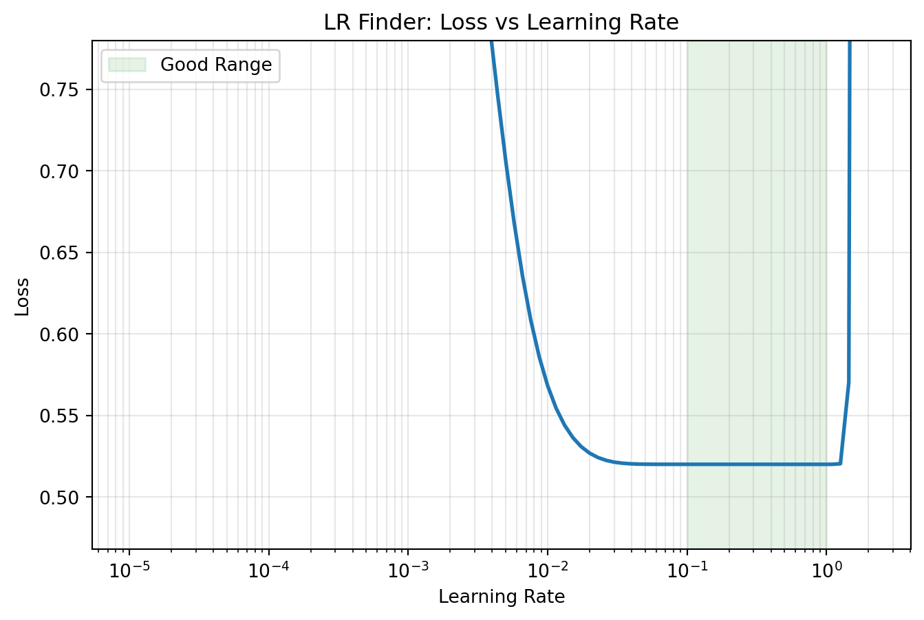
After running this routine, you plot Loss vs. Log Learning Rate.

• Flat region: The learning rate is too small; parameters aren’t moving.
• Steep drop: The learning rate is just right; the loss is decreasing rapidly.
• Rise/Explosion: The learning rate is too large; the model is diverging.

The Golden Rule: You do not pick the learning rate with the minimum loss on this plot (that is edging too close to instability). Instead, you pick a value in the middle of the steep drop, typically about 10x smaller than the point where the loss starts to rise.

Let’s run this diagnostic on our “Narrow Valley” problem:

Code

# -----------------------------
# Implementation of LR Finder
# -----------------------------

# configuration
lr_start = 1e-5
lr_end = 10.0
num_steps = 100

# Calculate multiplicative factor gamma
# lr_start * (gamma ** num_steps) = lr_end
gamma = (lr_end / lr_start) ** (1 / num_steps)

# Reset parameters to the starting point of the valley
w = np.array([-1.0, 0.25]) 

history_lr = []
history_loss = []
lr = lr_start

for t in range(num_steps):
    # 1. Compute Loss and Gradient
    loss = logistic_loss(w, X, y)
    grad = logistic_grad(w, X, y)
    
    # 2. Record
    history_loss.append(loss)
    history_lr.append(lr)
    
    # 3. Basic Stop Condition (if loss explodes)
    if t > 0 and loss > 4 * history_loss[0]:
        break
        
    # 4. Update Weights
    w = w - lr * grad
    
    # 5. Increase LR
    lr *= gamma

# -----------------------------
# Plotting the diagnostic
# -----------------------------
plt.figure(figsize=(8, 5))
plt.plot(history_lr, history_loss, linewidth=2)
plt.xscale('log')
plt.xlabel("Learning Rate")
plt.ylabel("Loss")
plt.title("LR Finder: Loss vs Learning Rate")
plt.grid(True, which="both", alpha=0.3)

# Limit y-axis to see the "valley" clearly (ignore explosion)
min_loss = min(history_loss)
plt.ylim(min_loss * 0.9, min_loss * 1.5)

# Annotate the "sweet spot"
# Roughly the steepest point before the minimum
plt.axvspan(1e-1, 1, color='green', alpha=0.1, label="Good Range")
plt.legend()

plt.show()

This plot shows a viable range of learning rates between .1 and 1. Somewhat surprisingly, this echoes what we saw previously that this learning rate range is where convergence in the ill-conditioned problem occurs!

---

Why this works surprisingly well

Despite its simplicity, the LR finder works because:

• most models have a broad stable range of learning rates,
• exact tuning is rarely necessary,
• being within the right order of magnitude matters far more than precision.

---

Learning rate schedules

The LR finder works pretty well, but we previously saw that \eta = .1 takes forever to get where we want it to go! On the other side, \eta = 1 gets there quickly but passes the minimum because the learning rate is too large to settle in at the actual minimum. A common way to cut the difference is to use a decaying learning rate schedule where the learning rate starts relatively large and decreases over time as GD approaches the minimum.

Three common decay schedules are exponential decay and cosine decay:

1. Exponential Decay: The learning rate is multiplied by a constant factor \gamma < 1 at every step (or epoch). \eta_t = \eta_0 \times \gamma^t This is simple but requires tuning \gamma carefully. If \gamma is too small, you stop learning too early; if too large, you never cool down.

2. Cosine Decay: The learning rate follows a cosine curve, starting at \eta_{max} and smoothly dropping to 0 (or \eta_{min}) by the end of training. \eta_t = \frac{1}{2}\eta_{max} \left(1 + \cos\left(\frac{t}{T}\pi\right)\right) This is standard in modern training (e.g., “Cosine Annealing”) because it maintains a high learning rate for a massive portion of training before dropping sharply and landing softly at the very end.

3. Step Decay: The learning rate is cut by a factor (e.g., cut in half) at fixed intervals. This is like downshifting a car; it allows the optimizer to “max out” its progress at a high speed, and then immediately stabilize by dropping to a lower speed.

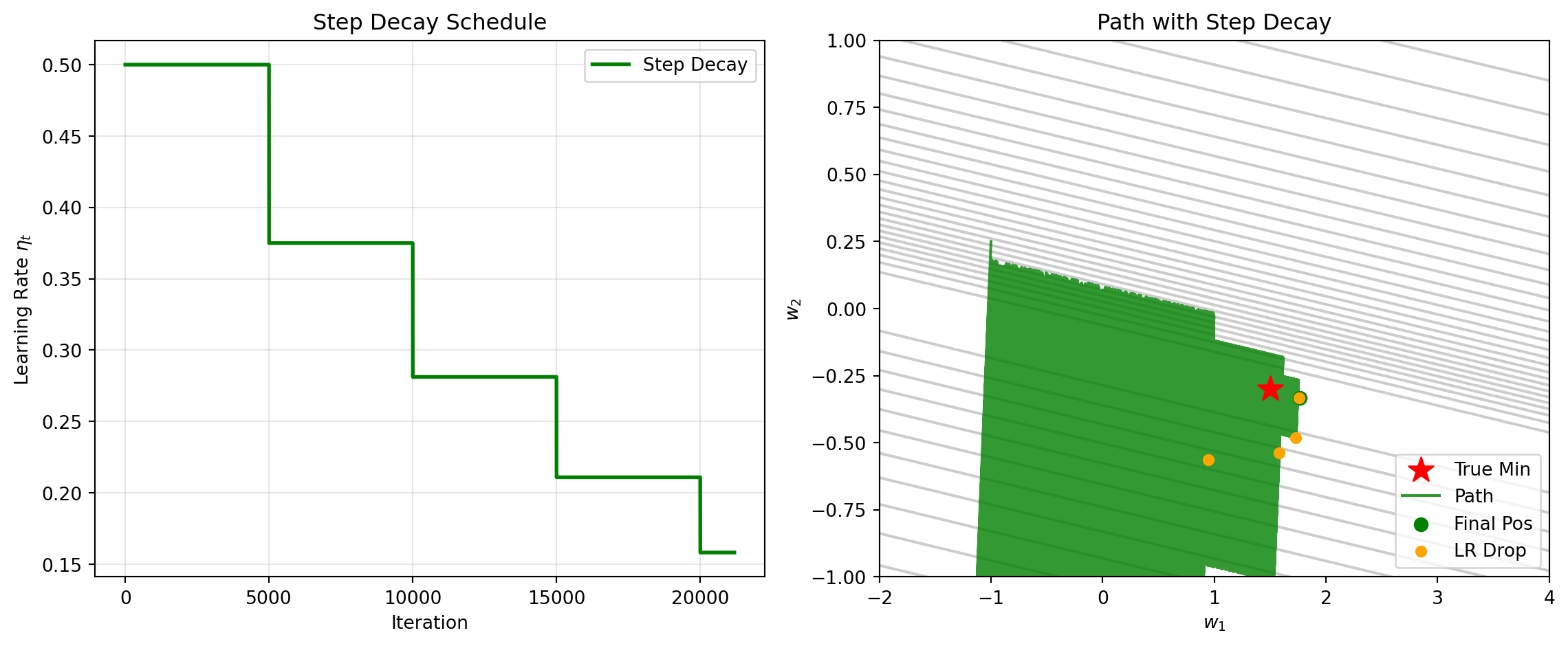
For ill-conditioned problems like our Narrow Valley, Step Decay is often superior. Let’s start with a very aggressive learning rate (\eta=.5) and multiply it by .75 every 5,000 steps.

Code

# -----------------------------
# Demonstration: Step Decay Application
# -----------------------------

# Settings
w = np.array([-1.0, 0.25]) # Start in the bad spot
max_iter = 100000

# Step Decay Configuration
lr_start = .5
drop_every = 5000
drop_factor = 0.75

# Tracking
path_step = [w.copy()]
lrs_step = []

for t in range(max_iter):
    grad = logistic_grad(w, X, y)
    
    # Step Decay Formula
    # Integer division // determines how many "drops" have occurred
    eta = lr_start * (drop_factor ** (t // drop_every))
    lrs_step.append(eta)
    
    w = w - eta * grad
    path_step.append(w.copy())
    
    # Early stop check (strict)
    if np.linalg.norm(grad) < 1e-5:
        break

path_step = np.array(path_step)

# -----------------------------
# Plotting the Comparison
# -----------------------------
plt.figure(figsize=(12, 5))

# Subplot 1: The Schedule
plt.subplot(1, 2, 1)
plt.plot(lrs_step, label="Step Decay", color='green', linewidth=2)
plt.xlabel("Iteration")
plt.ylabel("Learning Rate $\eta_t$")
plt.title("Step Decay Schedule")
plt.grid(True, alpha=0.3)
plt.legend()

# Subplot 2: The Path
plt.subplot(1, 2, 2)
# Background
plt.contour(W1, W2, Z, levels=np.logspace(np.log10(Z.min()), np.log10(Z.max()), 30), colors='gray', alpha=0.4)
plt.scatter(w_true[0], w_true[1], c='red', marker='*', s=200, label='True Min', zorder=10)

# Plot path
plt.plot(path_step[:, 0], path_step[:, 1], 'green', linewidth=1.5, alpha=0.8, label="Path")
plt.scatter(path_step[-1, 0], path_step[-1, 1], c='green', s=50, label='Final Pos')

# Mark the points where LR dropped
drop_indices = [i * drop_every for i in range(1, max_iter // drop_every + 1) if i * drop_every < len(path_step)]
if drop_indices:
    plt.scatter(path_step[drop_indices, 0], path_step[drop_indices, 1], 
                c='orange', marker='o', s=30, zorder=5, label='LR Drop')

plt.xlim(-2, 4)
plt.ylim(-1, 1)
plt.xlabel("$w_1$")
plt.ylabel("$w_2$")
plt.title("Path with Step Decay")
plt.legend(loc='lower right')
plt.tight_layout()
plt.show()

print(f"Final Step Decay Position: {path_step[-1]}")
print(f"Iterations taken: {len(path_step)}")

Final Step Decay Position: [ 1.76260406 -0.33185587]
Iterations taken: 21189

Implementing this strategy reduces the number of iterations needed to get to the minimum by half representing a significant time save!

---

Why schedules help

Early in training:

• parameters are far from optimal,
• large steps help explore.

Later in training:

• parameters are near a minimum,
• small steps prevent oscillation.

---

The deeper limitation of gradient descent

Even with a perfect learning rate and a smart schedule, standard Gradient Descent still struggles with our “narrow valley” problem. Why?

It comes down to a fundamental limitation: Gradient Descent treats every direction the same.

Imagine you are hiking down a narrow canyon.

• The path leading down the length of the canyon (towards the destination) is very gentle and flat.
• The walls on the sides of the canyon are incredibly steep.

Gradient Descent decides its step size based on the steepest slope it sees. In this canyon, the steepest slope is always the canyon walls, not the gentle path forward.

1. It sees the steep wall and takes a big jump away from it.
2. But because the wall is so steep, that jump overshoots and lands on the opposite wall.
3. From the opposite wall, it sees another steep slope and jumps back.
4. It ends up bouncing back and forth between the walls (zig-zagging), while making only tiny progress down the gentle path towards the actual minimum.

This is the “blindness” of standard Gradient Descent: it doesn’t know that the steep direction (the walls) is useless, and the flat direction (the path) is the one that matters.

Because it uses the same step size (\eta) for both directions, it is stuck in a dilemma:

• If \eta is big enough to move down the canyon, it’s too big for the walls (causing oscillation).
• If \eta is small enough to stop oscillating on the walls, it’s too tiny to move down the canyon (causing slow convergence).

This geometric mismatch is why simple Gradient Descent is rarely used on its own for complex deep learning problems. We need algorithms that can “see” the shape of the canyon.

---

Looking ahead

In the next sections, we will see how modern optimization addresses these issues:

• Second-order methods explicitly uses the Hessian to respond to curvature information but are limited by computational scaling limitations
• Momentum smooths oscillations
• Adaptive methods rescale gradients automatically

Gradient descent is the foundation—but not the endpoint. When gradient descent is combined with these three approaches, we get state of the art optimization machines!

---

Self-check questions

1. Why does ill-conditioning cause zig-zag behavior?
2. Why does the LR finder only need to be approximately correct?