Shape check: if \mathbf{x}\in\mathbb{R}^n, then H\in\mathbb{R}^{n\times n}.
Visualizing gradient and curvature in 2D
We’ll use a quadratic objective as our “microscope”:
f(\mathbf{x}) = \frac{1}{2}\mathbf{x}^\top A \mathbf{x}.
Quadratics are special because: - \nabla f(\mathbf{x}) = A\mathbf{x} - H(\mathbf{x}) = A (constant everywhere)
So this is the cleanest way to see what gradients and Hessians do.
Code
import numpy as npimport matplotlib.pyplot as pltdef quad_f(A, X, Y): Z = np.zeros_like(X)for i inrange(X.shape[0]):for j inrange(X.shape[1]): v = np.array([X[i, j], Y[i, j]]) Z[i, j] =0.5* v.T @ A @ vreturn Zdef plot_contour_and_grad(A, title, xlim=(-3,3), ylim=(-3,3)): x = np.linspace(xlim[0], xlim[1], 121) y = np.linspace(ylim[0], ylim[1], 121) X, Y = np.meshgrid(x, y) Z = quad_f(A, X, Y)# Gradient field: grad f = A x U = np.zeros_like(X) V = np.zeros_like(Y)for i inrange(X.shape[0]):for j inrange(X.shape[1]): v = np.array([X[i,j], Y[i,j]]) g = A @ v U[i,j], V[i,j] = g[0], g[1] plt.figure(figsize=(6,5)) cs = plt.contour(X, Y, Z, levels=18) plt.clabel(cs, inline=1, fontsize=8) step =10 plt.quiver(X[::step,::step], Y[::step,::step], U[::step,::step], V[::step,::step], angles='xy', scale_units='xy', scale=20) plt.title(title) plt.xlabel("$x_1$") plt.ylabel("$x_2$") plt.axhline(0, linewidth=0.8) plt.axvline(0, linewidth=0.8) plt.gca().set_aspect('equal', adjustable='box') plt.show()def curvature_along_direction(A, u, tmax=3.0, num=200, title=""): u = np.array(u, dtype=float) u = u / np.linalg.norm(u) ts = np.linspace(-tmax, tmax, num) vals = np.array([0.5* (t*u).T @ A @ (t*u) for t in ts]) curv = u.T @ A @ u plt.figure(figsize=(6,3.8)) plt.plot(ts, vals) plt.title(title +f"\nDirectional curvature $u^T H u = {curv:.2f}$") plt.xlabel("$t$ (moving along direction $u$)") plt.ylabel("$f(tu)$") plt.axhline(0, linewidth=0.8) plt.axvline(0, linewidth=0.8) plt.show()
Case 1: A bowl (local minimum)
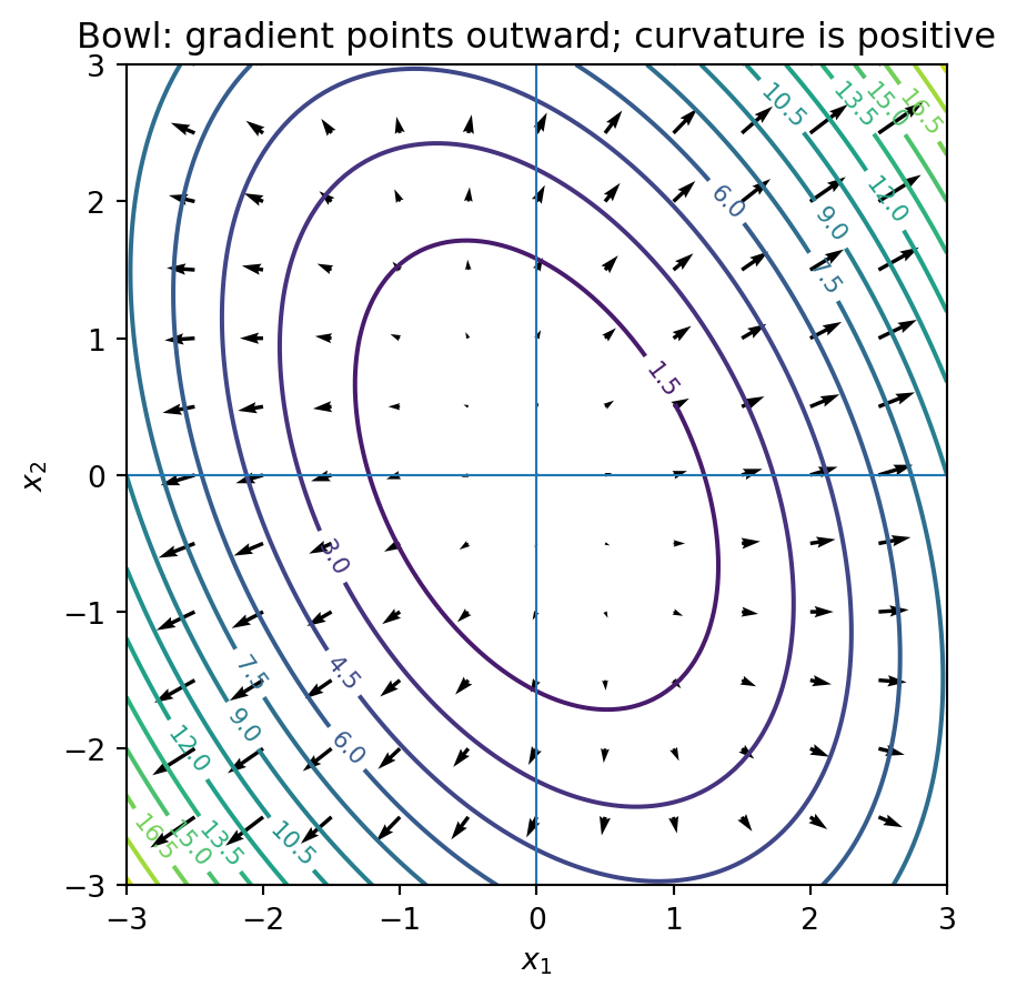
A bowl means curvature is positive in every direction.
Code
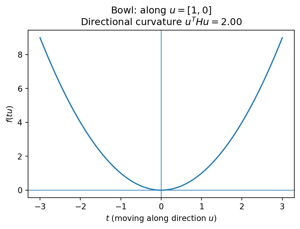
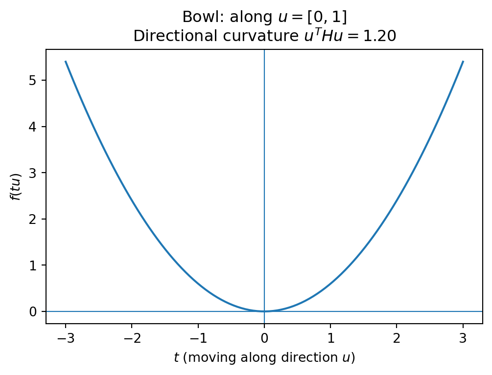
A_bowl = np.array([[2.0, 0.6], [0.6, 1.2]])plot_contour_and_grad(A_bowl, "Bowl: gradient points outward; curvature is positive")curvature_along_direction(A_bowl, u=[1,0], title="Bowl: along $u=[1,0]$")curvature_along_direction(A_bowl, u=[0,1], title="Bowl: along $u=[0,1]$")
Interpretation:
Gradient arrows point away from the origin (because the origin is the minimum).
Along any direction u, the 1D slice f(tu) is U-shaped.
Case 2: A saddle
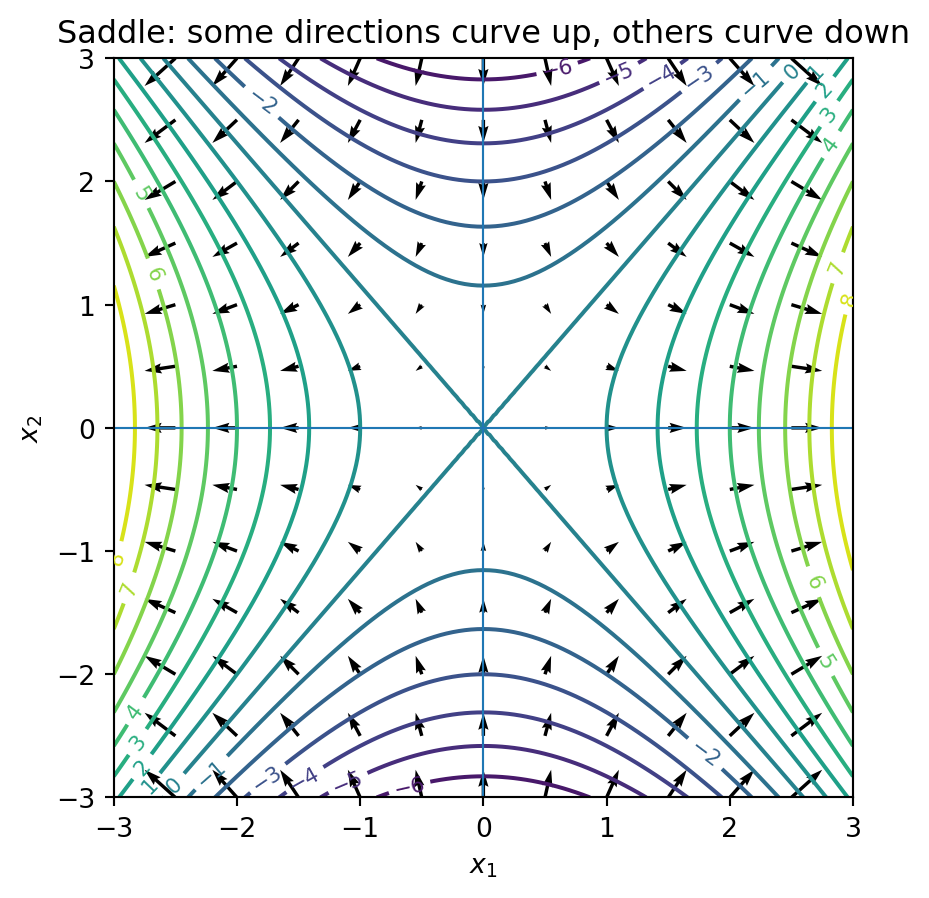
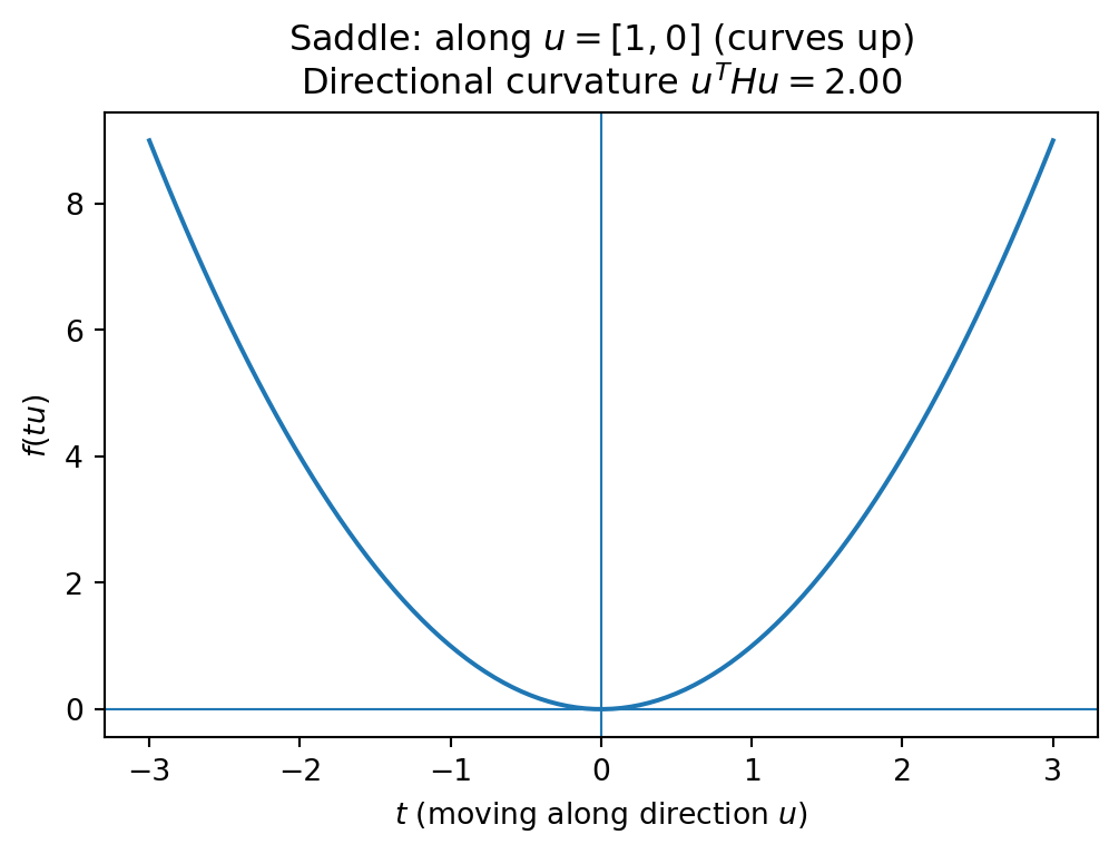
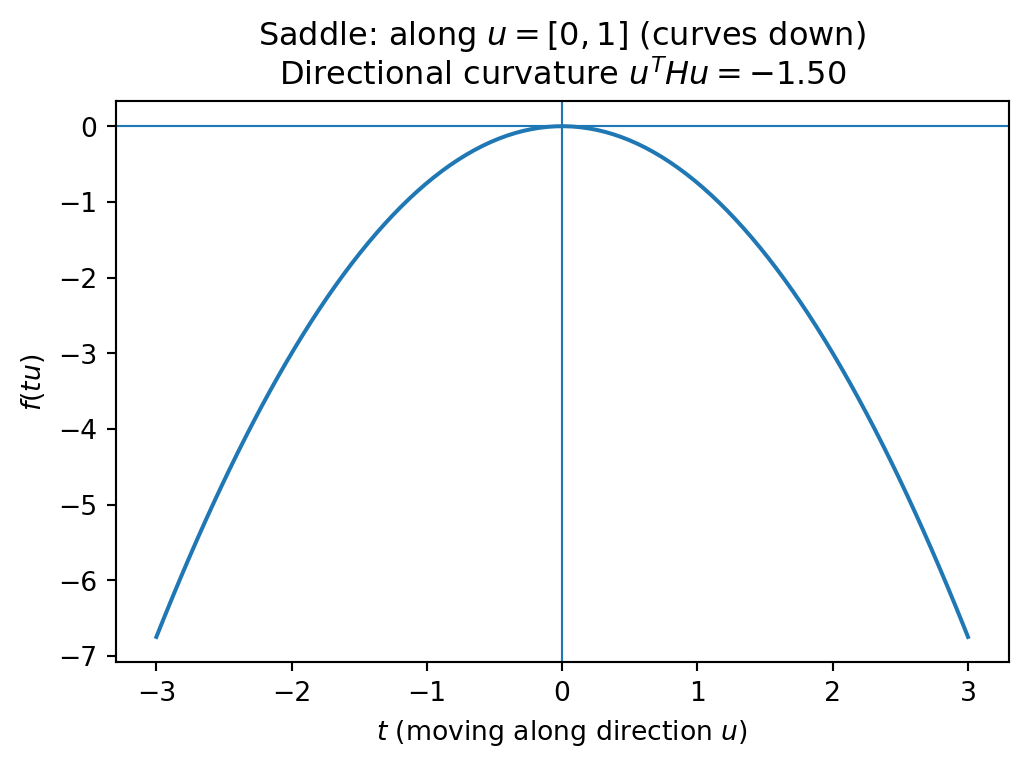
A saddle means curvature is positive in some directions and negative in others.
Code
A_saddle = np.array([[2.0, 0.0], [0.0, -1.5]])plot_contour_and_grad(A_saddle, "Saddle: some directions curve up, others curve down")curvature_along_direction(A_saddle, u=[1,0], title="Saddle: along $u=[1,0]$ (curves up)")curvature_along_direction(A_saddle, u=[0,1], title="Saddle: along $u=[0,1]$ (curves down)")
Interpretation:
Moving in one direction increases the function (bowl-like),
moving in another direction decreases it (hill-like),
so \nabla f = 0 does not imply a minimum.
Case 3: A ridge / flat direction
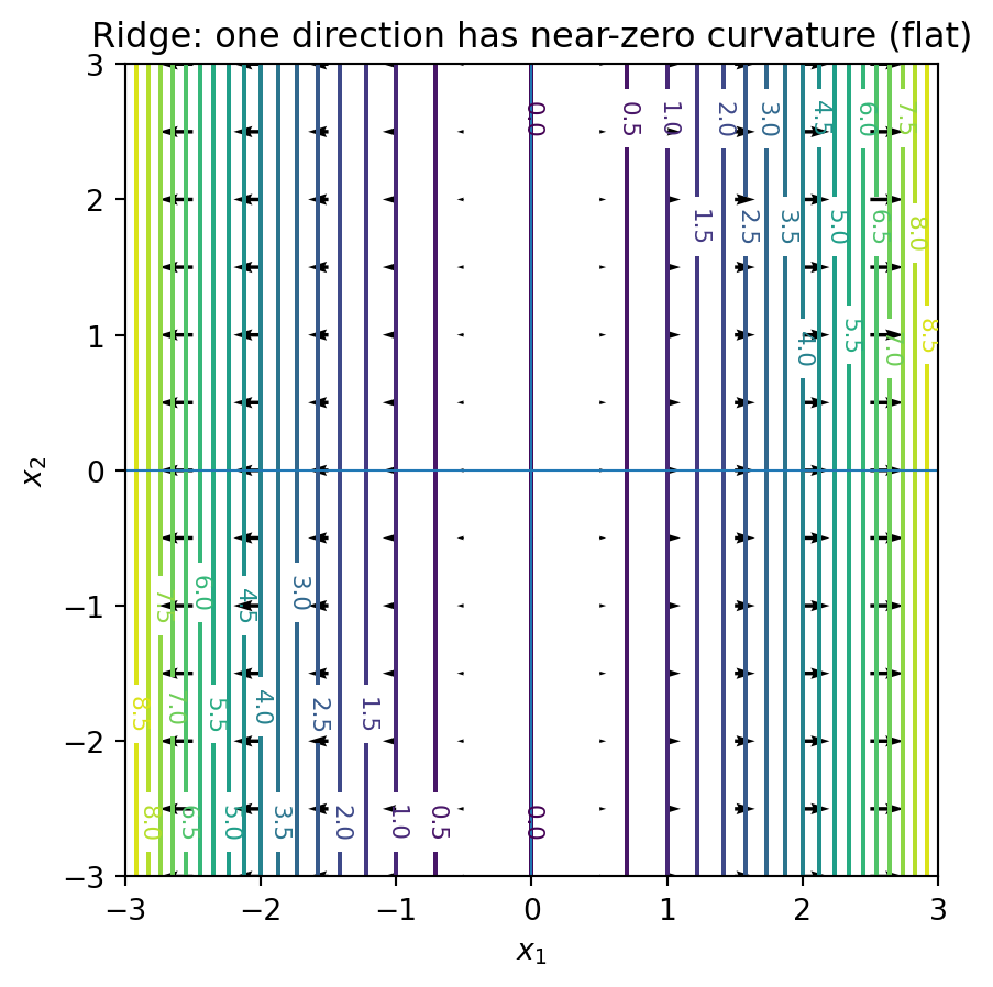
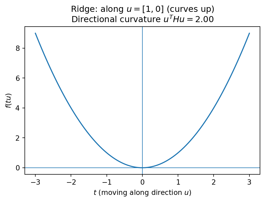
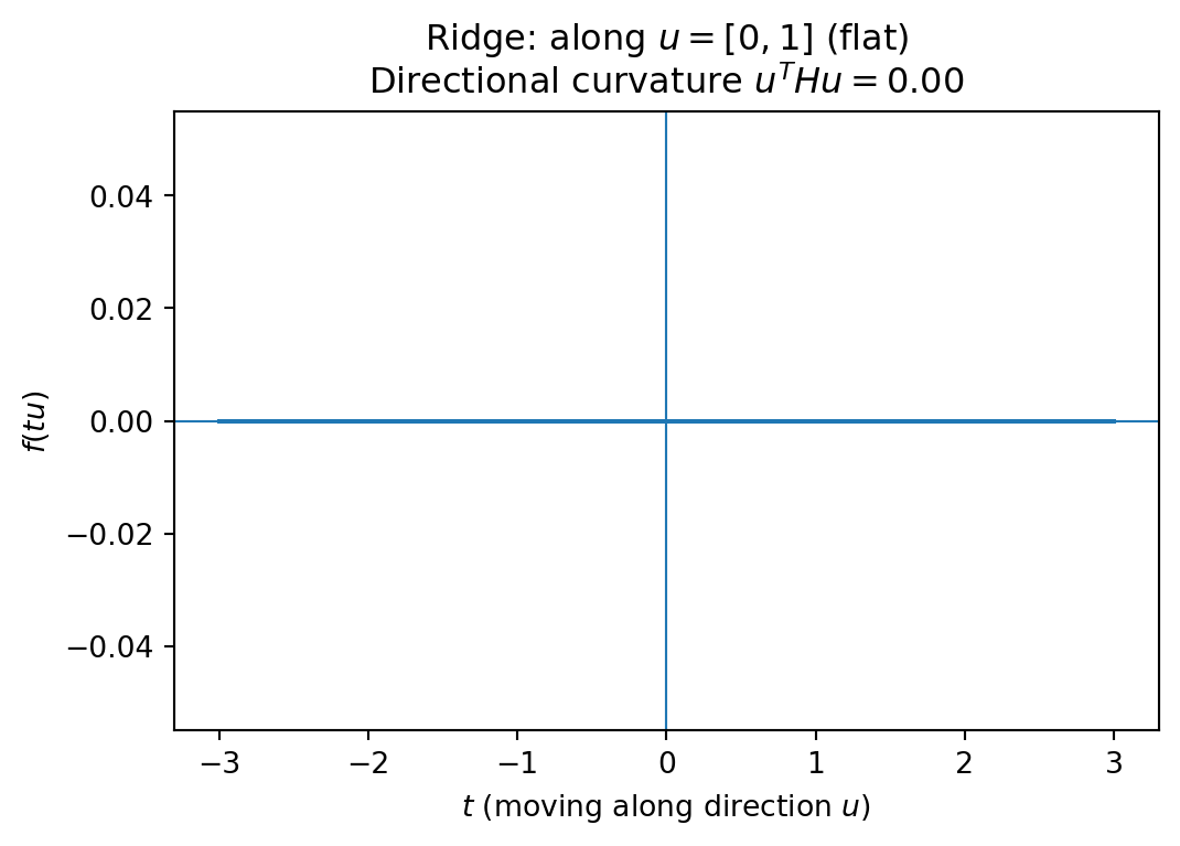
A ridge means there is at least one direction with (near) zero curvature.
Code
A_ridge = np.array([[2.0, 0.0], [0.0, 0.0]])plot_contour_and_grad(A_ridge, "Ridge: one direction has near-zero curvature (flat)")curvature_along_direction(A_ridge, u=[1,0], title="Ridge: along $u=[1,0]$ (curves up)")curvature_along_direction(A_ridge, u=[0,1], title="Ridge: along $u=[0,1]$ (flat)")
Interpretation:
Along one axis you see curvature,
along the other axis the function doesn’t change.
What the Hessian tells you (without starting from eigenvalues)
So the Hessian answers: “If I take a tiny step in direction \mathbf{u}, does the function bend upward or downward?”
\mathbf{u}^\top H \mathbf{u} > 0 for every \mathbf{u}\neq 0\Rightarrow local minimum
\mathbf{u}^\top H \mathbf{u} < 0 for every \mathbf{u}\neq 0\Rightarrow local maximum
sign depends on \mathbf{u}\Rightarrow saddle
\mathbf{u}^\top H \mathbf{u}=0 for some nonzero \mathbf{u}\Rightarrow flat direction
Where eigenvalues fit (one sentence)
Eigenvectors are the directions where curvature is “pure,” and eigenvalues are the corresponding curvatures.
But the practical test is the sign of \mathbf{u}^\top H \mathbf{u}.
H \succeq 0 but singular \Rightarrow ridge / flat directions
In Part 8, Newton’s method will use H to “precondition” the gradient—taking larger steps in low-curvature directions and smaller steps in high-curvature directions.
Key takeaways
The gradient points in the direction of steepest ascent.
The Hessian encodes local curvature.
Directional curvature \mathbf{u}^\top H \mathbf{u} is the most intuitive way to understand second derivatives.
Logistic regression has a positive semi-definite Hessian, so its loss is convex.
Self-check questions
If \nabla f(\mathbf{x}) = 0 and H(\mathbf{x}) = I, what kind of point is \mathbf{x}?
What is the shape of the Jacobian for a function mapping \mathbb{R}^3 \to \mathbb{R}^2?
In words: what does the quantity \mathbf{u}^\top H(\mathbf{x}) \mathbf{u} tell you about the function near \mathbf{x}?
Source Code
---title: "02: Gradients, Jacobians, and Hessians"format: html: code-fold: truejupyter: python3---# Why this mattersOptimization is navigation. A loss function $L(\theta)$ defines a landscape over parameter space.- The **gradient** tells us the local direction of steepest *increase* (so $-\nabla L$ is steepest descent).- The **Hessian** tells us local **curvature**—whether we are in a bowl, on a ridge, or near a saddle.In later notes, we will use these objects to build:- Gradient Descent updates: $\theta \leftarrow \theta - \eta \nabla L(\theta)$- Newton updates: $\theta \leftarrow \theta - H(\theta)^{-1}\nabla L(\theta)$So before we optimize anything, we need to be precise about what these derivatives *are* and what shapes they have.---# Definitions & ShapesAssume $\mathbf{x} \in \mathbb{R}^n$.## Gradient (Scalar $\to$ Vector)For $f: \mathbb{R}^n \to \mathbb{R}$, the gradient is the vector of partial derivatives:$$\nabla f(\mathbf{x}) =\begin{bmatrix}\frac{\partial f}{\partial x_1}\\\vdots\\\frac{\partial f}{\partial x_n}\end{bmatrix}\in \mathbb{R}^n.$$**Shape check:** scalar output $\Rightarrow$ gradient lives in the same space as the input.---## Jacobian (Vector $\to$ Vector)For a vector-valued function $\mathbf{f}: \mathbb{R}^n \to \mathbb{R}^m$, the Jacobian is an $m \times n$ matrix:$$J_{ij} = \frac{\partial f_i}{\partial x_j}.$$**Shape check:** output dimension by input dimension.---## Hessian (Scalar $\to$ Matrix)For $f: \mathbb{R}^n \to \mathbb{R}$, the Hessian is the matrix of second derivatives:$$H_{ij} = \frac{\partial^2 f}{\partial x_i \partial x_j}.$$When $f$ is smooth, $H$ is symmetric.**Shape check:** if $\mathbf{x}\in\mathbb{R}^n$, then $H\in\mathbb{R}^{n\times n}$.---# Visualizing gradient and curvature in 2DWe’ll use a quadratic objective as our “microscope”:$$f(\mathbf{x}) = \frac{1}{2}\mathbf{x}^\top A \mathbf{x}.$$Quadratics are special because:- $\nabla f(\mathbf{x}) = A\mathbf{x}$- $H(\mathbf{x}) = A$ (constant everywhere)So this is the cleanest way to see what gradients and Hessians *do*.```{python}import numpy as npimport matplotlib.pyplot as pltdef quad_f(A, X, Y): Z = np.zeros_like(X)for i inrange(X.shape[0]):for j inrange(X.shape[1]): v = np.array([X[i, j], Y[i, j]]) Z[i, j] =0.5* v.T @ A @ vreturn Zdef plot_contour_and_grad(A, title, xlim=(-3,3), ylim=(-3,3)): x = np.linspace(xlim[0], xlim[1], 121) y = np.linspace(ylim[0], ylim[1], 121) X, Y = np.meshgrid(x, y) Z = quad_f(A, X, Y)# Gradient field: grad f = A x U = np.zeros_like(X) V = np.zeros_like(Y)for i inrange(X.shape[0]):for j inrange(X.shape[1]): v = np.array([X[i,j], Y[i,j]]) g = A @ v U[i,j], V[i,j] = g[0], g[1] plt.figure(figsize=(6,5)) cs = plt.contour(X, Y, Z, levels=18) plt.clabel(cs, inline=1, fontsize=8) step =10 plt.quiver(X[::step,::step], Y[::step,::step], U[::step,::step], V[::step,::step], angles='xy', scale_units='xy', scale=20) plt.title(title) plt.xlabel("$x_1$") plt.ylabel("$x_2$") plt.axhline(0, linewidth=0.8) plt.axvline(0, linewidth=0.8) plt.gca().set_aspect('equal', adjustable='box') plt.show()def curvature_along_direction(A, u, tmax=3.0, num=200, title=""): u = np.array(u, dtype=float) u = u / np.linalg.norm(u) ts = np.linspace(-tmax, tmax, num) vals = np.array([0.5* (t*u).T @ A @ (t*u) for t in ts]) curv = u.T @ A @ u plt.figure(figsize=(6,3.8)) plt.plot(ts, vals) plt.title(title +f"\nDirectional curvature $u^T H u = {curv:.2f}$") plt.xlabel("$t$ (moving along direction $u$)") plt.ylabel("$f(tu)$") plt.axhline(0, linewidth=0.8) plt.axvline(0, linewidth=0.8) plt.show()```## Case 1: A bowl (local minimum)A bowl means curvature is positive in every direction.```{python}A_bowl = np.array([[2.0, 0.6], [0.6, 1.2]])plot_contour_and_grad(A_bowl, "Bowl: gradient points outward; curvature is positive")curvature_along_direction(A_bowl, u=[1,0], title="Bowl: along $u=[1,0]$")curvature_along_direction(A_bowl, u=[0,1], title="Bowl: along $u=[0,1]$")```Interpretation:- Gradient arrows point away from the origin (because the origin is the minimum).- Along any direction $u$, the 1D slice $f(tu)$ is U-shaped.---## Case 2: A saddleA saddle means curvature is positive in some directions and negative in others.```{python}A_saddle = np.array([[2.0, 0.0], [0.0, -1.5]])plot_contour_and_grad(A_saddle, "Saddle: some directions curve up, others curve down")curvature_along_direction(A_saddle, u=[1,0], title="Saddle: along $u=[1,0]$ (curves up)")curvature_along_direction(A_saddle, u=[0,1], title="Saddle: along $u=[0,1]$ (curves down)")```Interpretation:- Moving in one direction increases the function (bowl-like),- moving in another direction decreases it (hill-like),- so $\nabla f = 0$ does *not* imply a minimum.---## Case 3: A ridge / flat directionA ridge means there is at least one direction with (near) zero curvature.```{python}A_ridge = np.array([[2.0, 0.0], [0.0, 0.0]])plot_contour_and_grad(A_ridge, "Ridge: one direction has near-zero curvature (flat)")curvature_along_direction(A_ridge, u=[1,0], title="Ridge: along $u=[1,0]$ (curves up)")curvature_along_direction(A_ridge, u=[0,1], title="Ridge: along $u=[0,1]$ (flat)")```Interpretation:- Along one axis you see curvature,- along the other axis the function doesn’t change.---# What the Hessian tells you (without starting from eigenvalues)The key quantity is the **directional curvature**:$$\frac{d^2}{dt^2} f(\mathbf{x}+t\mathbf{u})\Big|_{t=0}= \mathbf{u}^\top H(\mathbf{x}) \mathbf{u}.$$So the Hessian answers: **“If I take a tiny step in direction $\mathbf{u}$, does the function bend upward or downward?”**- $\mathbf{u}^\top H \mathbf{u} > 0$ for every $\mathbf{u}\neq 0$ $\Rightarrow$ local minimum - $\mathbf{u}^\top H \mathbf{u} < 0$ for every $\mathbf{u}\neq 0$ $\Rightarrow$ local maximum - sign depends on $\mathbf{u}$ $\Rightarrow$ saddle - $\mathbf{u}^\top H \mathbf{u}=0$ for some nonzero $\mathbf{u}$ $\Rightarrow$ flat direction::: {.callout-note}## Where eigenvalues fit (one sentence)Eigenvectors are the directions where curvature is “pure,” and eigenvalues are the corresponding curvatures. But the practical test is the sign of $\mathbf{u}^\top H \mathbf{u}$.:::---# Connection to Optimization1. **Stationary points** satisfy $\nabla f(\mathbf{x}) = \mathbf{0}$.2. **Classification using the Hessian**: - $H \succ 0$ $\Rightarrow$ local minimum - $H \prec 0$ $\Rightarrow$ local maximum - $H$ indefinite $\Rightarrow$ saddle - $H \succeq 0$ but singular $\Rightarrow$ ridge / flat directionsIn Part 8, Newton’s method will use $H$ to “precondition” the gradient—taking larger steps in low-curvature directions and smaller steps in high-curvature directions.---# Key takeaways- The **gradient** points in the direction of steepest ascent.- The **Hessian** encodes local curvature.- Directional curvature $\mathbf{u}^\top H \mathbf{u}$ is the most intuitive way to understand second derivatives.- Logistic regression has a positive semi-definite Hessian, so its loss is convex.---# Self-check questions1. If $\nabla f(\mathbf{x}) = 0$ and $H(\mathbf{x}) = I$, what kind of point is $\mathbf{x}$?2. What is the shape of the Jacobian for a function mapping $\mathbb{R}^3 \to \mathbb{R}^2$?3. In words: what does the quantity $\mathbf{u}^\top H(\mathbf{x}) \mathbf{u}$ tell you about the function near $\mathbf{x}$?