In classical statistics, if you have a model with P=1,000,000 parameters and N=50,000 data points, you would expect massive overfitting. The model should memorize the training data and fail completely on test data.
As we saw in the previous tab, the noise in stochastic gradient descent allows the optimizer to escape sharp minima and travel towards flat minima which are more likely to generalize well.
It turns out that SGD is not just an optimization algorithm; it is also a Regularizer.
Even without adding an explicit penalty term (like +\lambda \|w\|^2) to our loss function, the dynamics of SGD implicitly prefer solutions with small norms in the same way as L2 regularization!
1. The Stochastic Differential Equation (SDE) View
To understand why SGD works differently than standard Gradient Descent, we need to stop looking at it as an algorithm and start looking at it as a physical process.
The standard SGD update rule is: w_{t+1} = w_t - \eta \tilde{g}(w_t)
where \tilde{g}(w_t) is the stochastic gradient calculated on a mini-batch. We can mathematically decompose this into two parts: the True Gradient (signal) and the variance of the mini-batch (noise).
If we imagine taking smaller and smaller steps (\eta \to 0) but taking more of them, this discrete process turns into a continuous curve described by a Stochastic Differential Equation (SDE):
This equation describes a particle moving through a landscape, influenced by two forces:
The Drift Terms (-\nabla L): This is Gravity.
It pulls the weights steadily downhill towards the nearest minimum.
In full-batch Gradient Descent, this is the only term that exists.
The Diffusion Term (\sqrt{\dots} dB_t): This is Temperature (Heat).
dB_t represents Brownian Motion—random jittering in all directions.
Crucially, the magnitude of this jitter is determined by the Learning Rate (\eta) and the Noise Covariance (\Sigma).
2. Explicit link to Ridge Regression
Let’s look at the noise covariance \Sigma(w_t). The noise comes from the variability of gradients across the mini-batch.
For a linear model (Least Squares), the noise covariance is proportional to the Hessian H: \Sigma \approx H
If we analyze the stationary distribution of this SDE, the term acts like a penalty. Specifically, Smith & Le (2018) showed that maximizing the probability path of this SDE is equivalent to minimizing a modified loss function:
\min_w L(w) + \frac{\eta}{4B} \| \nabla L(w) \|^2
\eta: Learning Rate
B: Batch Size
This is called Implicit Gradient Regularization. SGD penalizes sharp regions of the loss function (where \| \nabla L(w) \|^2 is large) and prefers flat regions.
Connection to Minimum Norm
For over-parameterized linear regression initialized at zero, SGD converges to the specific solution that solves Xw=y while minimizing the L2 Euclidean Norm\|w\|_2.
\min \|w\|_2 \quad \text{subject to} \quad Xw = y
This is exactly what Ridge Regression (L2 Regularization) tries to achieve explicitly!
3. SGD as Implicit Regularization
Together, all of this implies a recipe that allows SGD to find generalizable solutions that mimic those that would be given adding explicit L2 regularization to our loss function:
Use SGD with a small (but not too small) learning rate
Use SGD with a small (but not too small) batch size
Initialize all unknown parameters at or close to zero
What this means is that fitting models using SGD will seek out more generalizable solution through:
Avoiding sharp minima
Choosing solutions that mimic that of a Ridge penalty
4. Simulation: Infinite Solutions
Let’s simulate an over-parameterized problem. * Data: N=50 samples. * Features: P=100 dimensions. * True Model: Only 2 features matter. The other 98 are noise (but correlated noise).
In this overparameterized scenario, there are an infinite number of solutions to this system that have exactly zero loss.
However, there is one solution that we think is best because it represents the simplest model:
The Minimum Norm Solution: The solution w^* that satisfies the equations but has the smallest possible length (\|w\|_2). This corresponds to the solution found by Ridge Regression (as \lambda \to 0).
It turns out that SGD starting at \mathbf 0 will find this point! The connection actually runs even deeper:
Let the path of solutions defined by a Ridge regression solution be given as the set of coefficients that minimize the following objective: \underset{\mathbf w^*}{\min} L(\mathbf w; \mathbf x, y) - \lambda \|\mathbf w \|^2 where \lambda is the standard Ridge tuning parameter for all values of \lambda between 0 and \infty
Define the coefficient path for SGD under the same loss function without the Ridge penalty with sufficiently small \eta as the steps SGD takes from its starting point at \mathbf 0 to its final converged location.
These two paths will be startingly similar!
Code
import numpy as npimport matplotlib.pyplot as pltfrom sklearn.decomposition import PCAfrom sklearn.linear_model import Ridgenp.random.seed(42)# 1. Setup Over-parameterized Linear ProblemN =50P =100Z = np.random.randn(N, P)Cov = np.random.randn(P, P)X = Z @ CovX = (X - X.mean(axis=0)) / (X.std(axis=0) +1e-8)w_true = np.zeros(P)w_true[0] =3.0w_true[1] =-2.0y = X @ w_true + np.random.randn(N) *0.1# 2. Compute Ridge Path (Lambda: Infinity -> Zero)# We use logspace to span a huge range of lambdaslambdas = np.logspace(4, -5, 100)ridge_path = []for lam in lambdas: model = Ridge(alpha=lam, fit_intercept=False) model.fit(X, y) ridge_path.append(model.coef_)ridge_path = np.array(ridge_path)# 3. Compute SGD Path (Time: 0 -> Max)# Use a very small learning rate to approximate continuous gradient floww = np.zeros(P)sgd_path = [w.copy()]lr =0.001steps =10000for _ inrange(steps):# Full batch for cleaner visualization to match theory, # but works with mini-batch too (just noisier) grad = X.T @ (X @ w - y) w = w - lr * grad sgd_path.append(w.copy())sgd_path = np.array(sgd_path)# 4. Visualization via PCA# Combine data to learn common projectioncombined_data = np.vstack([ridge_path, sgd_path])pca = PCA(n_components=2)all_pca = pca.fit_transform(combined_data)n_ridge =len(ridge_path)p_ridge = all_pca[0:n_ridge]p_sgd = all_pca[n_ridge:]plt.figure(figsize=(10, 6))# Plot Ridge Trajectoryplt.plot(p_ridge[:,0], p_ridge[:,1], 'r--', linewidth=3, label=r"Ridge Path ($\lambda: \infty \to 0$)")# Mark direction of Ridgeplt.arrow(p_ridge[10,0], p_ridge[10,1], p_ridge[11,0]-p_ridge[10,0], p_ridge[11,1]-p_ridge[10,1], color='red', head_width=0.05)# Plot SGD Trajectoryplt.plot(p_sgd[:,0], p_sgd[:,1], 'b-', linewidth=2, alpha=0.7, label=r"Gradient Descent ($t: 0 \to \infty$)")# Mark direction of SGDplt.arrow(p_sgd[100,0], p_sgd[100,1], p_sgd[105,0]-p_sgd[100,0], p_sgd[105,1]-p_sgd[100,1], color='blue', head_width=0.05)# Start Pointplt.scatter(p_sgd[0,0], p_sgd[0,1], c='black', s=100, marker='o', label="Start (0,0)")plt.title("The Equivalence of Optimization Time and Regularization Strength")plt.xlabel("PC1")plt.ylabel("PC2")plt.legend()plt.grid(True, alpha=0.3)plt.show()
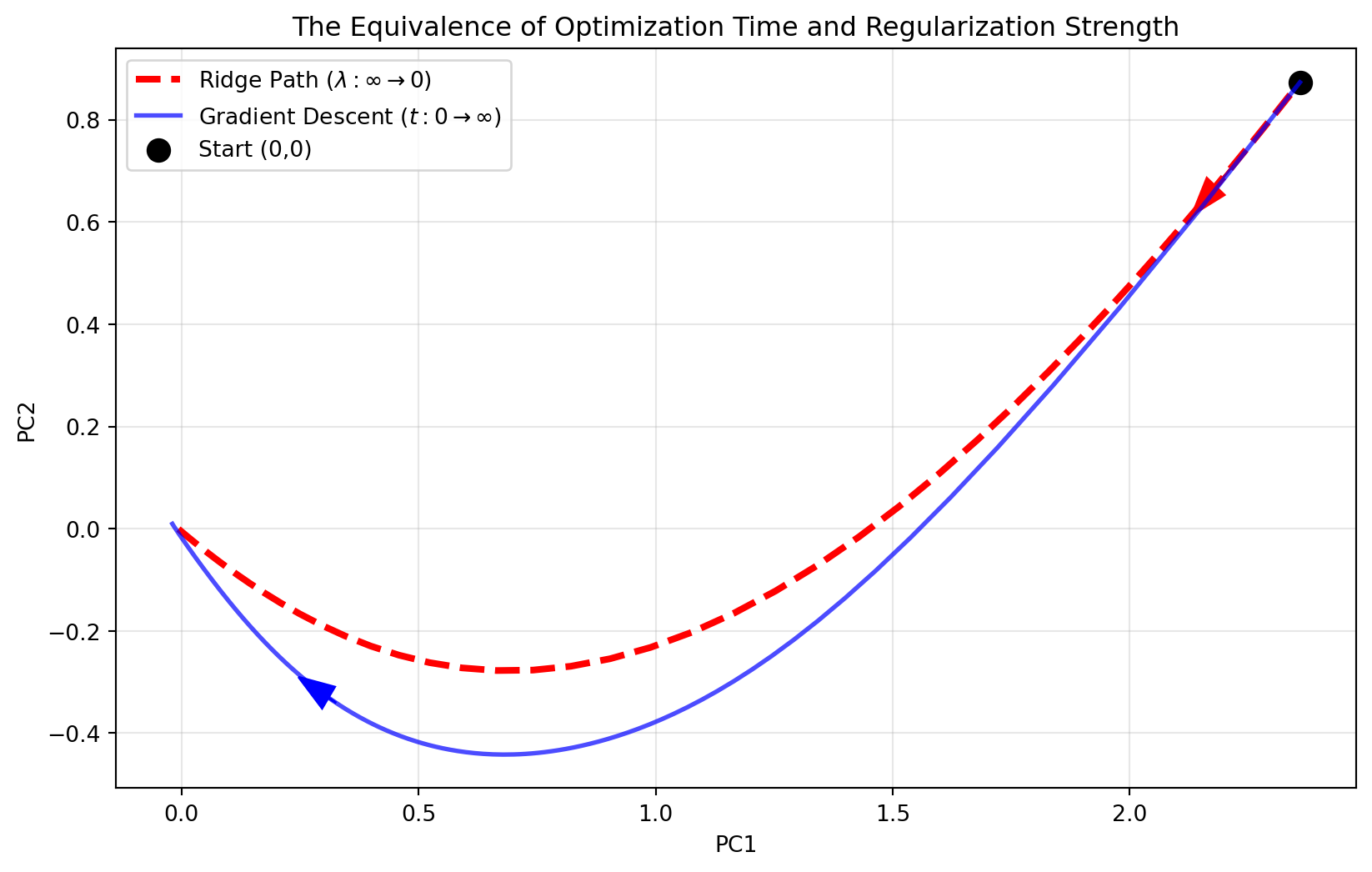
The plot above shows the Ridge path and the SGD path in a reduced dimensionality space given by the first two principal components.
The Red Dashed Line is the set of all optimal solutions for every possible Ridge penalty \lambda.
The Blue Solid Line is the path taken by the optimizer over time.
They are nearly identical! This confirms a fundamental intuition in Deep Learning theory: Time is a Regularizer.
Stopping early (t is small) is mathematically equivalent to high regularization (\lambda is large).
Running forever (t \to \infty) corresponds to zero regularization (\lambda \to 0).
5. Early Stopping as Implicit Regularization
The simulation above leads us directly to one of the most practical “hacks” in Deep Learning: Early Stopping.
If training for a long time decreases the “effective regularization” (driving the implicit \lambda \to 0) and allows complexity to grow, then we can control complexity simply by stopping the training process before it converges!
The Mechanism
Start at Zero: The model starts with effectively infinite regularization (w=0). The complexity is minimal.
Training Begins: As iterations proceed, the weights grow. The “effective \lambda” drops. The model starts learning the simplest, most dominant patterns in the data (large principal components).
The Sweet Spot: At some iteration t^*, the effective regularization strength is optimal for the Test Data. The model has captured the signal but not the noise.
Overfitting Begins: As t \to \infty, the implicit \lambda becomes too small. The optimizer obsessively chases the tiny residual errors in the training set (noise), driving the test error up.
Much like Ridge regression and Lasso, we need to come up with a method that will allow us to choose when to stop. The most common way to do this is with a single train/validation split: use 80% of our training data to learn the gradients and use 20% of the data to check the out-of-sample performance of our model at each step.
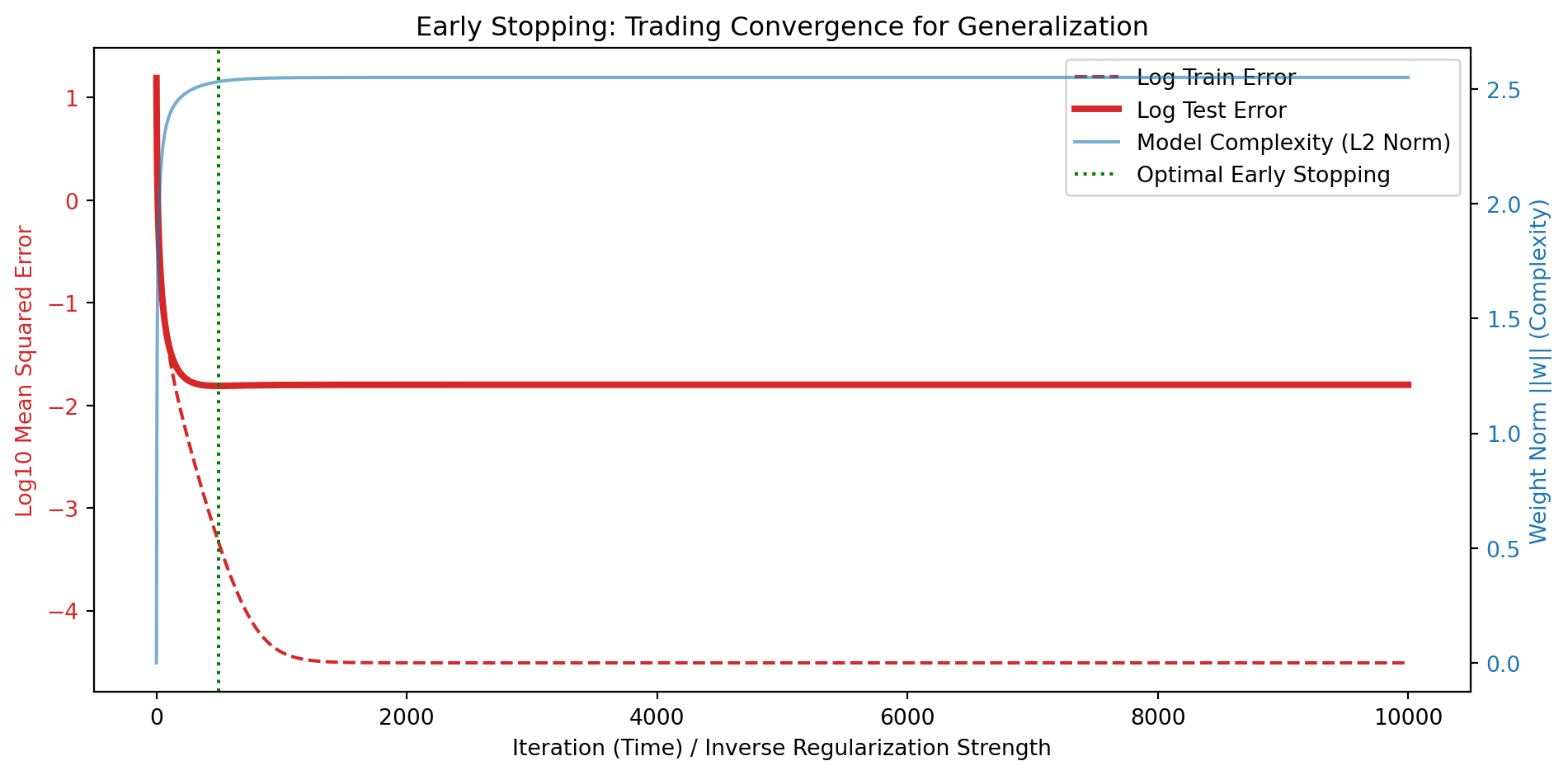
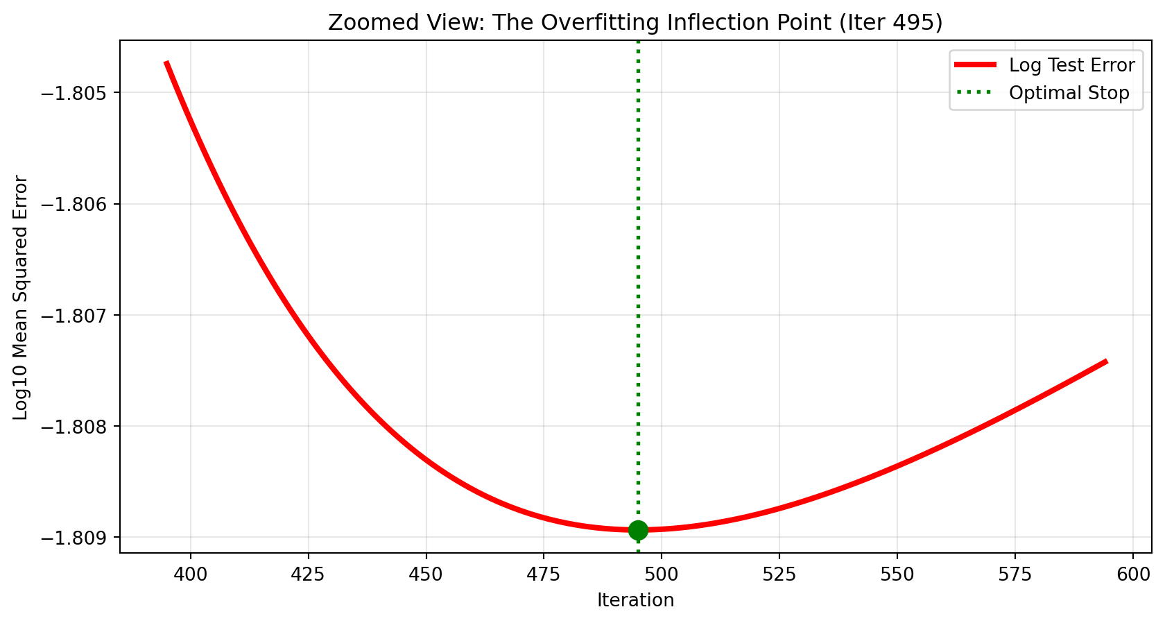
The main idea is that early in the SGD process we’re severely underfitting and our validation loss will be high. As time proceeds (or as we loosen the regularization), our validation loss improves. At a certain point, though, we’ll hit the inflection point where our validation loss begins to increase again (overfitting). This is when we want to stop!
Simulation: The Validation “U-Shape”
Let’s verify this by checking the Validation Error on our over-parameterized dataset. We will track the Test Error and the Norm of the weights (Complexity) as training progresses.
Code
# 1. Generate Test Datay_test = X @ w_true + np.random.randn(N) *0.1# Same X, new noise for generalization test# 2. Track Train vs Test Error along the SGD pathtrain_errs = []test_errs = []norms = []for w_curr in sgd_path: # using the path computed in prev block# Train MSE tr_pred = X @ w_curr train_errs.append(np.mean((tr_pred - y)**2))# Test MSE (Generalization) te_pred = X @ w_curr test_errs.append(np.mean((te_pred - y_test)**2))# L2 Norm norms.append(np.linalg.norm(w_curr))# 3. Plotfig, ax1 = plt.subplots(figsize=(10, 5))color ='tab:red'ax1.set_xlabel('Iteration (Time) / Inverse Regularization Strength')ax1.set_ylabel('Log10 Mean Squared Error', color=color) # PLOTTING THE LOG OF THE ERRORS NOW# We capture the line objects to build a custom legend laterlns1 = ax1.plot(np.log10(train_errs), color=color, linestyle='--', label="Log Train Error")lns2 = ax1.plot(np.log10(test_errs), color=color, linewidth=3, label="Log Test Error")ax1.tick_params(axis='y', labelcolor=color)ax2 = ax1.twinx() # instantiate a second axes that shares the same x-axiscolor ='tab:blue'ax2.set_ylabel('Weight Norm ||w|| (Complexity)', color=color) lns3 = ax2.plot(norms, color=color, alpha=0.6, label="Model Complexity (L2 Norm)")ax2.tick_params(axis='y', labelcolor=color)# Find minimum test errormin_test_idx = np.argmin(test_errs)stop_line = ax1.axvline(min_test_idx, color='green', linestyle=':', label="Optimal Early Stopping")# Combine all legends from ax1, ax2, and the vertical linelns = lns1 + lns2 + lns3 + [stop_line]labs = [l.get_label() for l in lns]ax1.legend(lns, labs, loc='upper right')plt.title("Early Stopping: Trading Convergence for Generalization")fig.tight_layout() plt.show()print(f"Optimal Stopping Iteration: {min_test_idx}")# 4. Zoomed-In Plot around the Minimumzoom_window =100start_idx =max(0, min_test_idx - zoom_window)end_idx =min(len(test_errs), min_test_idx + zoom_window)steps_zoom = np.arange(start_idx, end_idx)fig, ax = plt.subplots(figsize=(10, 5))# Plot Test Error in the zoomed windowax.plot(steps_zoom, np.log10([test_errs[i] for i in steps_zoom]), color='red', linewidth=3, label="Log Test Error")# Mark the minimumax.axvline(min_test_idx, color='green', linestyle=':', linewidth=2, label="Optimal Stop")ax.scatter(min_test_idx, np.log10(test_errs[min_test_idx]), color='green', s=100, zorder=5)ax.set_xlabel('Iteration')ax.set_ylabel('Log10 Mean Squared Error')ax.set_title(f"Zoomed View: The Overfitting Inflection Point (Iter {min_test_idx})")ax.legend()ax.grid(True, alpha=0.3)plt.show()
Optimal Stopping Iteration: 495
The optimal model is NOT found where the gradient is zero (t \to \infty). The optimal model is found “on the way” there. By stopping early, we implicitly chose the specific regularization strength that generalizes best.
Source Code
---title: "14: Implicit Regularization of Stochastic Gradient Descent"format: html: code-fold: truejupyter: python3---## The Mystery of GeneralizationIn classical statistics, if you have a model with $P=1,000,000$ parameters and $N=50,000$ data points, you would expect massive **overfitting**. The model should memorize the training data and fail completely on test data.Yet, Deep Neural Networks ($\text{Parameters} \gg \text{Data}$) generalize remarkably well. Why?As we saw in the previous tab, the noise in stochastic gradient descent allows the optimizer to escape sharp minima and travel towards flat minima which are more likely to generalize well.It turns out that **SGD is not just an optimization algorithm; it is also a Regularizer.**Even without adding an explicit penalty term (like $+\lambda \|w\|^2$) to our loss function, the dynamics of SGD *implicitly* prefer solutions with small norms in the same way as L2 regularization!---## 1. The Stochastic Differential Equation (SDE) ViewTo understand why SGD works differently than standard Gradient Descent, we need to stop looking at it as an algorithm and start looking at it as a **physical process**.The standard SGD update rule is:$$ w_{t+1} = w_t - \eta \tilde{g}(w_t) $$where $\tilde{g}(w_t)$ is the stochastic gradient calculated on a mini-batch. We can mathematically decompose this into two parts: the **True Gradient** (signal) and the **variance** of the mini-batch (noise).$$ \tilde{g}(w_t) = \underbrace{\nabla L(w_t)}_{\text{Signal}} + \underbrace{\epsilon_t}_{\text{Noise}} $$If we imagine taking smaller and smaller steps ($\eta \to 0$) but taking more of them, this discrete process turns into a continuous curve described by a **Stochastic Differential Equation (SDE)**:$$ dW_t = \underbrace{-\nabla L(W_t) dt}_{\text{Drift}} + \underbrace{\sqrt{\frac{\eta}{B} \Sigma(W_t)} dB_t}_{\text{Diffusion}} $$### Breaking it DownThis equation describes a particle moving through a landscape, influenced by two forces:1. **The Drift Terms ($-\nabla L$)**: This is **Gravity**. * It pulls the weights steadily downhill towards the nearest minimum. * In full-batch Gradient Descent, this is the *only* term that exists.2. **The Diffusion Term ($\sqrt{\dots} dB_t$)**: This is **Temperature (Heat)**. * $dB_t$ represents Brownian Motion—random jittering in all directions. * Crucially, the magnitude of this jitter is determined by the **Learning Rate ($\eta$)** and the **Noise Covariance ($\Sigma$)**.---## 2. Explicit link to Ridge RegressionLet's look at the noise covariance $\Sigma(w_t)$. The noise comes from the variability of gradients across the mini-batch.For a linear model (Least Squares), the noise covariance is proportional to the Hessian $H$:$$ \Sigma \approx H $$If we analyze the stationary distribution of this SDE, the term acts like a penalty. Specifically, Smith & Le (2018) showed that maximizing the probability path of this SDE is equivalent to minimizing a modified loss function:$$ \min_w L(w) + \frac{\eta}{4B} \| \nabla L(w) \|^2 $$* $\eta$: Learning Rate* $B$: Batch SizeThis is called **Implicit Gradient Regularization**. SGD penalizes **sharp** regions of the loss function (where $\| \nabla L(w) \|^2$ is large) and prefers **flat** regions.### Connection to Minimum NormFor over-parameterized linear regression initialized at zero, SGD converges to the specific solution that solves $Xw=y$ while minimizing the **L2 Euclidean Norm** $\|w\|_2$.$$ \min \|w\|_2 \quad \text{subject to} \quad Xw = y $$This is exactly what **Ridge Regression** (L2 Regularization) tries to achieve explicitly!---## 3. SGD as Implicit RegularizationTogether, all of this implies a recipe that allows SGD to find generalizable solutions that mimic those that would be given adding explicit L2 regularization to our loss function:1. Use SGD with a small (but not too small) learning rate2. Use SGD with a small (but not too small) batch size3. Initialize all unknown parameters at or close to zeroWhat this means is that fitting models using SGD will seek out more generalizable solution through:- Avoiding sharp minima- Choosing solutions that mimic that of a Ridge penalty---## 4. Simulation: Infinite SolutionsLet's simulate an over-parameterized problem.* **Data**: $N=50$ samples.* **Features**: $P=100$ dimensions.* **True Model**: Only 2 features matter. The other 98 are noise (but correlated noise).In this overparameterized scenario, there are an infinite number of solutions to this system that have exactly zero loss.However, there is one solution that we think is best because it represents the **simplest model**:**The Minimum Norm Solution**: The solution $w^*$ that satisfies the equations but has the smallest possible length ($\|w\|_2$). This corresponds to the solution found by **Ridge Regression** (as $\lambda \to 0$).It turns out that SGD starting at $\mathbf 0$ will find this point! The connection actually runs even deeper:1. Let the **path** of solutions defined by a Ridge regression solution be given as the set of coefficients that minimize the following objective:$$\underset{\mathbf w^*}{\min} L(\mathbf w; \mathbf x, y) - \lambda \|\mathbf w \|^2$$where $\lambda$ is the standard Ridge tuning parameter for all values of $\lambda$ between 0 and $\infty$ 2. Define the coefficient path for SGD under the same loss function without the Ridge penalty with sufficiently small $\eta$ as the steps SGD takes from its starting point at $\mathbf 0$ to its final converged location.These two paths will be **startingly similar**!```{python}import numpy as npimport matplotlib.pyplot as pltfrom sklearn.decomposition import PCAfrom sklearn.linear_model import Ridgenp.random.seed(42)# 1. Setup Over-parameterized Linear ProblemN =50P =100Z = np.random.randn(N, P)Cov = np.random.randn(P, P)X = Z @ CovX = (X - X.mean(axis=0)) / (X.std(axis=0) +1e-8)w_true = np.zeros(P)w_true[0] =3.0w_true[1] =-2.0y = X @ w_true + np.random.randn(N) *0.1# 2. Compute Ridge Path (Lambda: Infinity -> Zero)# We use logspace to span a huge range of lambdaslambdas = np.logspace(4, -5, 100)ridge_path = []for lam in lambdas: model = Ridge(alpha=lam, fit_intercept=False) model.fit(X, y) ridge_path.append(model.coef_)ridge_path = np.array(ridge_path)# 3. Compute SGD Path (Time: 0 -> Max)# Use a very small learning rate to approximate continuous gradient floww = np.zeros(P)sgd_path = [w.copy()]lr =0.001steps =10000for _ inrange(steps):# Full batch for cleaner visualization to match theory, # but works with mini-batch too (just noisier) grad = X.T @ (X @ w - y) w = w - lr * grad sgd_path.append(w.copy())sgd_path = np.array(sgd_path)# 4. Visualization via PCA# Combine data to learn common projectioncombined_data = np.vstack([ridge_path, sgd_path])pca = PCA(n_components=2)all_pca = pca.fit_transform(combined_data)n_ridge =len(ridge_path)p_ridge = all_pca[0:n_ridge]p_sgd = all_pca[n_ridge:]plt.figure(figsize=(10, 6))# Plot Ridge Trajectoryplt.plot(p_ridge[:,0], p_ridge[:,1], 'r--', linewidth=3, label=r"Ridge Path ($\lambda: \infty \to 0$)")# Mark direction of Ridgeplt.arrow(p_ridge[10,0], p_ridge[10,1], p_ridge[11,0]-p_ridge[10,0], p_ridge[11,1]-p_ridge[10,1], color='red', head_width=0.05)# Plot SGD Trajectoryplt.plot(p_sgd[:,0], p_sgd[:,1], 'b-', linewidth=2, alpha=0.7, label=r"Gradient Descent ($t: 0 \to \infty$)")# Mark direction of SGDplt.arrow(p_sgd[100,0], p_sgd[100,1], p_sgd[105,0]-p_sgd[100,0], p_sgd[105,1]-p_sgd[100,1], color='blue', head_width=0.05)# Start Pointplt.scatter(p_sgd[0,0], p_sgd[0,1], c='black', s=100, marker='o', label="Start (0,0)")plt.title("The Equivalence of Optimization Time and Regularization Strength")plt.xlabel("PC1")plt.ylabel("PC2")plt.legend()plt.grid(True, alpha=0.3)plt.show()```The plot above shows the Ridge path and the SGD path in a reduced dimensionality space given by the first two principal components.- The Red Dashed Line is the set of all optimal solutions for every possible Ridge penalty $\lambda$.- The Blue Solid Line is the path taken by the optimizer over time.They are nearly identical! This confirms a fundamental intuition in Deep Learning theory: Time is a Regularizer.- Stopping early ($t$ is small) is mathematically equivalent to high regularization ($\lambda$ is large).- Running forever ($t \to \infty$) corresponds to zero regularization ($\lambda \to 0$).## 5. Early Stopping as Implicit RegularizationThe simulation above leads us directly to one of the most practical "hacks" in Deep Learning: **Early Stopping**.If training for a long time decreases the "effective regularization" (driving the implicit $\lambda \to 0$) and allows complexity to grow, then we can control complexity simply by stopping the training process before it converges!### The Mechanism1. **Start at Zero**: The model starts with effectively infinite regularization ($w=0$). The complexity is minimal.2. **Training Begins**: As iterations proceed, the weights grow. The "effective $\lambda$" drops. The model starts learning the simplest, most dominant patterns in the data (large principal components).3. **The Sweet Spot**: At some iteration $t^*$, the effective regularization strength is optimal for the Test Data. The model has captured the signal but not the noise.4. **Overfitting Begins**: As $t \to \infty$, the implicit $\lambda$ becomes too small. The optimizer obsessively chases the tiny residual errors in the training set (noise), driving the test error up.Much like Ridge regression and Lasso, we need to come up with a method that will allow us to choose **when** to stop. The most common way to do this is with a single train/validation split: use 80% of our training data to learn the gradients and use 20% of the data to check the **out-of-sample** performance of our model at each step.The main idea is that early in the SGD process we're severely underfitting and our validation loss will be high. As time proceeds (or as we loosen the regularization), our validation loss improves. At a certain point, though, we'll hit the inflection point where our validation loss begins to increase again (overfitting). This is when we want to stop!### Simulation: The Validation "U-Shape"Let's verify this by checking the Validation Error on our over-parameterized dataset. We will track the Test Error and the Norm of the weights (Complexity) as training progresses.```{python}# 1. Generate Test Datay_test = X @ w_true + np.random.randn(N) *0.1# Same X, new noise for generalization test# 2. Track Train vs Test Error along the SGD pathtrain_errs = []test_errs = []norms = []for w_curr in sgd_path: # using the path computed in prev block# Train MSE tr_pred = X @ w_curr train_errs.append(np.mean((tr_pred - y)**2))# Test MSE (Generalization) te_pred = X @ w_curr test_errs.append(np.mean((te_pred - y_test)**2))# L2 Norm norms.append(np.linalg.norm(w_curr))# 3. Plotfig, ax1 = plt.subplots(figsize=(10, 5))color ='tab:red'ax1.set_xlabel('Iteration (Time) / Inverse Regularization Strength')ax1.set_ylabel('Log10 Mean Squared Error', color=color) # PLOTTING THE LOG OF THE ERRORS NOW# We capture the line objects to build a custom legend laterlns1 = ax1.plot(np.log10(train_errs), color=color, linestyle='--', label="Log Train Error")lns2 = ax1.plot(np.log10(test_errs), color=color, linewidth=3, label="Log Test Error")ax1.tick_params(axis='y', labelcolor=color)ax2 = ax1.twinx() # instantiate a second axes that shares the same x-axiscolor ='tab:blue'ax2.set_ylabel('Weight Norm ||w|| (Complexity)', color=color) lns3 = ax2.plot(norms, color=color, alpha=0.6, label="Model Complexity (L2 Norm)")ax2.tick_params(axis='y', labelcolor=color)# Find minimum test errormin_test_idx = np.argmin(test_errs)stop_line = ax1.axvline(min_test_idx, color='green', linestyle=':', label="Optimal Early Stopping")# Combine all legends from ax1, ax2, and the vertical linelns = lns1 + lns2 + lns3 + [stop_line]labs = [l.get_label() for l in lns]ax1.legend(lns, labs, loc='upper right')plt.title("Early Stopping: Trading Convergence for Generalization")fig.tight_layout() plt.show()print(f"Optimal Stopping Iteration: {min_test_idx}")# 4. Zoomed-In Plot around the Minimumzoom_window =100start_idx =max(0, min_test_idx - zoom_window)end_idx =min(len(test_errs), min_test_idx + zoom_window)steps_zoom = np.arange(start_idx, end_idx)fig, ax = plt.subplots(figsize=(10, 5))# Plot Test Error in the zoomed windowax.plot(steps_zoom, np.log10([test_errs[i] for i in steps_zoom]), color='red', linewidth=3, label="Log Test Error")# Mark the minimumax.axvline(min_test_idx, color='green', linestyle=':', linewidth=2, label="Optimal Stop")ax.scatter(min_test_idx, np.log10(test_errs[min_test_idx]), color='green', s=100, zorder=5)ax.set_xlabel('Iteration')ax.set_ylabel('Log10 Mean Squared Error')ax.set_title(f"Zoomed View: The Overfitting Inflection Point (Iter {min_test_idx})")ax.legend()ax.grid(True, alpha=0.3)plt.show()```The optimal model is NOT found where the gradient is zero ($t \to \infty$). The optimal model is found "on the way" there. By stopping early, we implicitly chose the specific regularization strength that generalizes best.