09: Momentum

The Problem with “Amnesia”

Standard Gradient Descent suffers from severe amnesia.

At every step t, it looks at the gradient \nabla L(w_t) and takes a step. Once the step is taken, it forgets everything. At step t+1, it starts from scratch.

This is why the “Narrow Valley” pathology is so devastating: 1. Step 1 says “Go steep left!” \rightarrow Jump left. 2. Step 2 says “Go steep right!” \rightarrow Jump right. 3. The algorithm never realizes, “Hey, I’ve been bouncing left and right for 100 steps, maybe I should stop doing that and focus on the forward motion?”

Newton’s Method fixed this by calculating curvature (\mathbf{H}^{-1}), effectively telling the algorithm regarding the shape ahead of time. But that costs O(d^3).

Momentum fixes this by giving the optimizer memory (specifically, velocity). It costs O(d), virtually free.

---

1. Physics Intuition: The Heavy Ball

Imagine optimization as rolling a ball down a hill.

• Gradient Descent behaves like a feather. It follows the wind (gradient) perfectly at every instant. If the wind changes direction, the feather changes direction instantly.
• Momentum behaves like a heavy bowling ball. It gains velocity.
  • If the gradient keeps pushing it down the valley, it gains speed (acceleration).
  • If the gradient tries to push it sideways (zig-zag), the ball’s existing forward momentum resists the sudden change.

The Algorithm

We introduce a velocity vector v, which accumulates the gradients over time.

\begin{align} v_{t+1} &= \underbrace{\beta v_t}_{\text{Friction}} + \underbrace{\eta \nabla L(w_t)}_{\text{Acceleration}} \\ w_{t+1} &= w_t - v_{t+1} \end{align}

• \beta: The momentum coefficient (usually 0.9). Think of this as friction or decay. It says “keep 90% of your previous speed.”
• \eta: The learning rate.

How it solves the “Zig-Zag”

Consider our valley walls:

• The gradients oscillate: +10, -10, +10, -10.
• The sum (velocity) averages out: +10 - 10 \approx 0.
• Result: The destructive oscillations cancel each other out.

Consider the valley floor:

• The gradients are small but consistent: 0.1, 0.1, 0.1, 0.1.
• The sum (velocity) builds up: 0.1 \to 0.2 \to 0.3 \dots
• Result: The constructive signal amplifies, allowing us to move fast even with small gradients.

---

2. Comparison: GD vs Newton vs Momentum

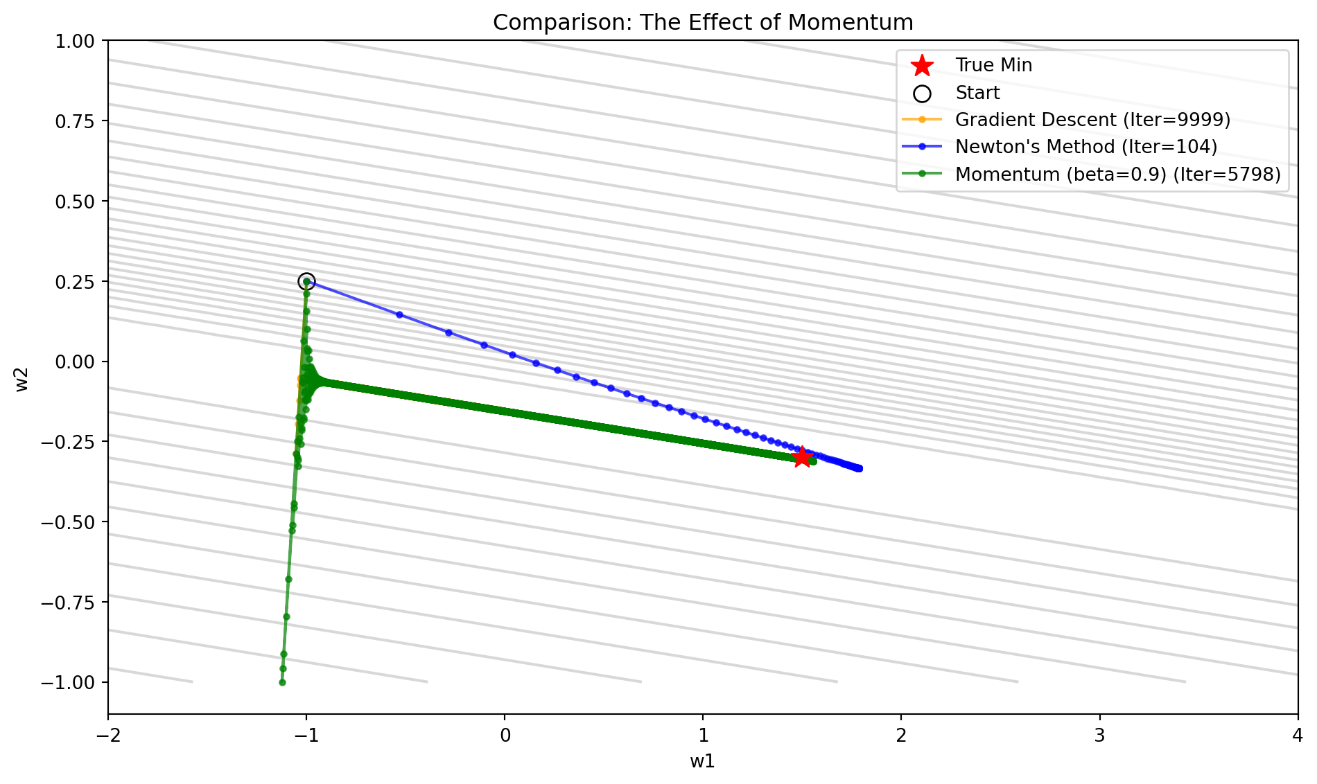
Let’s run our “Narrow Valley” torture test again. We will compare:

1. Gradient Descent: The baseline (\eta = 0.1).
2. Newton’s Method: The expensive ideal (\eta = 0.1).
3. Momentum: The cheap approximation (\eta = 0.1, \beta = 0.9).

Code

import numpy as np
import matplotlib.pyplot as plt
import time
from IPython.display import Markdown

# -----------------------------
# 1. Setup the Nasty Valley (Ill-conditioned)
# -----------------------------
np.random.seed(42)
n = 10_000

x1 = np.random.normal(0, 1, n)
x2 = 10.0 * x1 + np.random.normal(0, .5, n) 
X = np.column_stack([x1, x2])
w_true = np.array([1.5, -0.3]) 

logits = X @ w_true
p = 1 / (1 + np.exp(-logits))
y = np.random.binomial(1, p)

def get_loss(w):
    p = 1 / (1 + np.exp(-X @ w))
    eps = 1e-12
    return -np.average(y * np.log(p + eps) + (1 - y) * np.log(1 - p + eps))

def get_grad(w):
    p = 1 / (1 + np.exp(-X @ w))
    return (X.T @ (p - y)) / n

def get_hessian(w):
    p = 1 / (1 + np.exp(-X @ w))
    weights = p * (1 - p)
    return (X.T @ (weights[:, None] * X)) / n

# -----------------------------
# 2. Run Algorithms
# -----------------------------
w_start = np.array([-1.0, 0.25])
tol = 1e-4
max_iter = 10000 

results = []

# --- A. Gradient Descent ---
w = w_start.copy()
path_gd = [w.copy()]
start = time.time()
converged = False
for i in range(max_iter):
    grad = get_grad(w)
    if np.linalg.norm(grad) < tol: converged = True; break
    w = w - 0.1 * grad
    path_gd.append(w.copy())
results.append({"name": "Gradient Descent", "path": np.array(path_gd), "time": time.time()-start, "iters": i, "conv": converged})

# --- B. Newton's Method ---
w = w_start.copy()
path_newt = [w.copy()]
start = time.time()
converged = False
for i in range(max_iter):
    grad = get_grad(w)
    if np.linalg.norm(grad) < tol: converged = True; break
    H = get_hessian(w)
    try: step = np.linalg.solve(H, grad)
    except: break
    w = w - 0.1 * step # Learning rate 0.1
    path_newt.append(w.copy())
results.append({"name": "Newton's Method", "path": np.array(path_newt), "time": time.time()-start, "iters": i, "conv": converged})

# --- C. Momentum ---
w = w_start.copy()
v = np.zeros_like(w) # Velocity starts at 0
path_mom = [w.copy()]
start = time.time()
converged = False
beta = 0.9 # Momentum coefficient

for i in range(max_iter):
    grad = get_grad(w)
    if np.linalg.norm(grad) < tol: converged = True; break
    
    # Momentum Update
    v = beta * v + 0.1 * grad
    w = w - v
    
    path_mom.append(w.copy())
results.append({"name": "Momentum (beta=0.9)", "path": np.array(path_mom), "time": time.time()-start, "iters": i, "conv": converged})


# -----------------------------
# 3. Visualization
# -----------------------------
w1_vals = np.linspace(-2, 4, 100)
w2_vals = np.linspace(-1, 1, 100)
W1, W2 = np.meshgrid(w1_vals, w2_vals)
Z = np.zeros_like(W1)
for i in range(W1.shape[0]):
    for j in range(W1.shape[1]):
        Z[i,j] = get_loss(np.array([W1[i,j], W2[i,j]]))

plt.figure(figsize=(10, 6))
plt.contour(W1, W2, Z, levels=np.logspace(np.log10(Z.min()), np.log10(Z.max()), 30), colors='gray', alpha=0.3)
plt.scatter(w_true[0], w_true[1], c='red', marker='*', s=150, zorder=10, label="True Min")
plt.scatter(w_start[0], w_start[1], c='white', edgecolors='black', s=80, label="Start")

colors = ['orange', 'blue', 'green']
styles = ['o-', 'o-', 'o-']

for idx, res in enumerate(results):
    path = res['path']
    plt.plot(path[:,0], path[:,1], styles[idx], label=f"{res['name']} (Iter={res['iters']})", 
             color=colors[idx], markersize=3, alpha=0.7, linewidth=1.5)

plt.title("Comparison: The Effect of Momentum")
plt.xlabel("w1")
plt.ylabel("w2")
plt.legend()
plt.tight_layout()
plt.show()

# -----------------------------
# 4. Table
# -----------------------------
table_md = """
| Algorithm | Iterations | Total Time (s) | Time/Iter (ms) | Final w | Status |
|---|---|---|---|---|---|
"""
for res in results:
    s = "Converged ✅" if res['conv'] else "Slow ⏳"
    w_s = f"({res['path'][-1][0]:.3f}, {res['path'][-1][1]:.3f})"
    
    # Avoid division by zero
    iters = res['iters'] if res['iters'] > 0 else 1
    t_per_iter_ms = (res['time'] / iters) * 1000
    
    table_md += f"| {res['name']} | {res['iters']} | {res['time']:.4f} | {t_per_iter_ms:.4f} | {w_s} | {s} |\n"

Markdown(table_md)

Algorithm	Iterations	Total Time (s)	Time/Iter (ms)	Final w	Status
Gradient Descent	9999	0.4338	0.0434	(-0.045, -0.151)	Slow ⏳
Newton’s Method	104	0.0131	0.1262	(1.786, -0.334)	Converged ✅
Momentum (beta=0.9)	5798	0.2268	0.0391	(1.554, -0.311)	Converged ✅

Observations

1. Newton (Blue): Still the champion. It understands the geometry perfectly and takes the most direct path. Most expensive in terms of compute time per iteration.
2. Momentum (Green): A massive improvement over standard GD.
   • Look at the path: It overshoots slightly (like a real heavy ball swinging past the bottom), but the oscillations are damped.
   • It accelerates down the valley much faster than GD.
   • The time per iteration is essentially the same as gradient descent, but it effectively handles the slow zig-zag that plagues gradient descent.
3. Gradient Descent (Orange): Painfully slow, zig-zagging inefficiently.

Momentum successfully gives us the “Rotation” benefit of Newton’s method (smoothing the path) without calculating the Hessian.

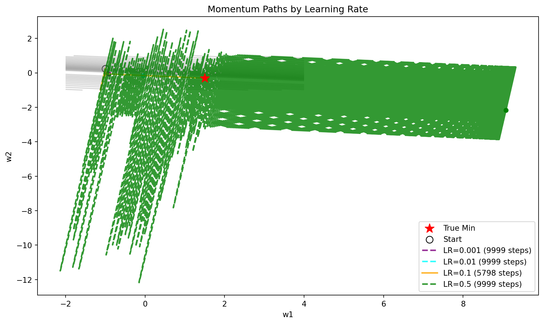
However, notice that Momentum still requires us to tune the learning rate carefully.

Code

# -----------------------------
# LR Sensitivity Test: Path Visualization
# -----------------------------
lrs = [0.001, 0.01, 0.1, 0.5]
results_lr = []

w_start = np.array([-1.0, 0.25])
tol = 1e-4
max_iter = 10000

for lr in lrs:
    w = w_start.copy()
    v = np.zeros_like(w)
    path = [w.copy()]
    converged = False
    start_time = time.time()
    
    for i in range(max_iter):
        grad = get_grad(w)
        loss = get_loss(w)
        
        # Divergence check
        if loss > 20 or np.isnan(loss):
            break
            
        if np.linalg.norm(grad) < tol:
            converged = True
            break
            
        v = 0.9 * v + lr * grad
        w = w - v
        path.append(w.copy())
        
    duration = time.time() - start_time
    results_lr.append({
        "lr": lr,
        "path": np.array(path),
        "iters": i,
        "time": duration,
        "converged": converged
    })

# -----------------------------
# 1. Visualization
# -----------------------------
plt.figure(figsize=(10, 6))
plt.contour(W1, W2, Z, levels=np.logspace(np.log10(Z.min()), np.log10(Z.max()), 30), colors='gray', alpha=0.3)
plt.scatter(w_true[0], w_true[1], c='red', marker='*', s=150, zorder=10, label="True Min")
plt.scatter(w_start[0], w_start[1], c='white', edgecolors='black', s=80, label="Start")

colors = ['purple', 'cyan', 'orange', 'green', 'red']

for idx, res in enumerate(results_lr):
    path = res['path']
    label = f"LR={res['lr']} ({res['iters']} steps)"
    
    # Use different line styles for variety
    ls = '-' if res['converged'] else '--'
    
    plt.plot(path[:,0], path[:,1], color=colors[idx % len(colors)], linestyle=ls, 
             linewidth=2, alpha=0.8, label=label)
    
    # Mark end
    plt.scatter(path[-1,0], path[-1,1], color=colors[idx % len(colors)], s=30)

plt.title("Momentum Paths by Learning Rate")
plt.xlabel("w1")
plt.ylabel("w2")
plt.legend()
plt.tight_layout()
plt.show()

# -----------------------------
# 2. Summary Table
# -----------------------------
table_md = """
| Learning Rate | Iterations | Time (s) | Final w | Status |
|---|---|---|---|---|
"""
for res in results_lr:
    s = "Converged ✅" if res['converged'] else "Diverged/Slow ❌"
    w_s = f"({res['path'][-1][0]:.3f}, {res['path'][-1][1]:.3f})"
    table_md += f"| {res['lr']} | {res['iters']} | {res['time']:.4f} | {w_s} | {s} |\n"

Markdown(table_md)

Learning Rate	Iterations	Time (s)	Final w	Status
0.001	9999	1.1684	(-0.912, -0.065)	Diverged/Slow ❌
0.01	9999	1.1498	(-0.046, -0.151)	Diverged/Slow ❌
0.1	5798	0.6233	(1.554, -0.311)	Converged ✅
0.5	9999	1.1258	(9.076, -2.163)	Diverged/Slow ❌

It doesn’t solve the Scale problem (different sensitivities for different parameters). For that, we need Adaptive Gradients.