For linear regression, we can solve for the optimal parameters in closed form.
For logistic regression, we cannot.
Even though the loss function is convex, there is no equation we can rearrange to obtain \mathbf w^\* directly.
Instead, we must search for the minimum.
This section introduces gradient descent as a geometric procedure for navigating a loss landscape. We will focus on binary logistic regression with two features so that we can see what the algorithm is doing.
This is the last time optimization will look this simple.
\nabla_{\mathbf w} L
=
\frac{1}{n}\mathbf X^\top(\mathbf p - \mathbf y).
Written out to show the full mapping of \mathbf X to \mathbf y:
\nabla_{\mathbf w} L
=
\frac{1}{n}\mathbf X^\top(\sigma(\mathbf X^\top \mathbf w) - \mathbf y).
where \sigma(\cdot) is the logistic function applied elementwise. Note that b is omitted here as we’re assuming that \mathbf X has a column of 1s.
We could try to solve for this analytically by finding \mathbf w^* such that:
\frac{1}{n}\mathbf X^\top(\sigma(\mathbf X^\top \mathbf w^*) - \mathbf y) = \mathbf 0
Unfortunately, this is not possible due to the pesky logistic function!
Instead, we’ll need to leverage an iterative optimization procedure to find the loss minimizing values of \mathbf w.
The gradient descent algorithm
Gradient descent is a first-order iterative optimization method.
Starting from an initial guess \mathbf w^{(0)}, we repeatedly apply
\nabla_{\mathbf w} L is evaluated at the current parameters.
Each update moves the parameters in the direction of steepest descent. In other words, gradient descent will move from any point to the point \eta away that maximally decreases loss
Why the negative gradient?
To understand why gradient descent works, let’s think about the most efficient move from the current parameter value, \mathbf w:
\underset{\mathbf d}{\max} L(\mathbf w) - L(\mathbf w + \eta\mathbf d)
where \eta is a very small positive value (almost zero!) and \mathbf d is a unit vector. \mathbf d controls the direction of the move of size \eta away from our current point.
In words, our goal is to find the direction away from the current position that maximizes the decrease in loss.
Step 1: Use a first-order approximation
Because \eta is tiny, we can use a first-order Taylor expansion around \mathbf w:
L(\mathbf w + \eta \mathbf d)
\approx
L(\mathbf w) + \eta \nabla L(\mathbf w)^\top \mathbf d.
Iterative Gradient Descent and Covergence Guarantees
Using this identity, an iterative strategy for finding a local minimum for any loss function for which we can evaluate the value of the gradient at any point arises:
Choose a starting point, \mathbf w^{(0)}, and a small step-size, \eta. Set t = 0.
Evaluate the gradient for the unknowns with respect to the loss at t: \nabla L(\mathbf w^{(t)})
This approach is guaranteed to find a local minimum eventually since each step is guaranteed to find a \mathbf w^{(t + 1)} that has weakly lower loss than the previous \mathbf w. If we are at a critical point (e.g. \nabla L(\mathbf w^{(t)}) = \mathbf 0), note that the update step goes to zero and we no longer move!
In practice, we can only guarantee convergence has occurred if the following to conditions are met:
t = \infty
\eta = \epsilon where \epsilon is the smallest positive number greater than 0
Unfortunately, neither of these conditions are practically achievable. Instead, we typically say that it’s “good enough” and ready to stop if one (or more) of the following conditions is met:
Relative loss change
\frac{|L^{(t)} - L^{(t-1)}|}{L^{(t-1)}} < \text{tol}
Maximum iterations (a safety bound)
All three reflect the same idea: we stop when further progress is negligible.
Gradient descent in action (binary logistic regression with two features)
Now we will watch gradient descent work in the simplest setting where we can actually see the loss landscape.
We will use:
two classes (y \in \{0,1\}),
two features (\mathbf x_i \in \mathbb R^2),
no intercept (b=0, so you can think of \mathbf X as already containing a column of ones if you want an intercept later),
and a ground-truth parameter vector
\mathbf w_{\text{true}} = \begin{bmatrix} 1 \\ -1 \end{bmatrix}.
This gives us a clean “sandbox” where:
We can visualize the data in (x_1, x_2) space.
We can visualize the loss surface in (w_1, w_2) space.
We can click anywhere in parameter space and see gradient descent walk to the minimum.
This is the last time optimization will feel like geometry on a 2D picture.
The goal is to build intuition here before we lose the ability to “see” the landscape.
Step 1: Simulate a dataset we can visualize
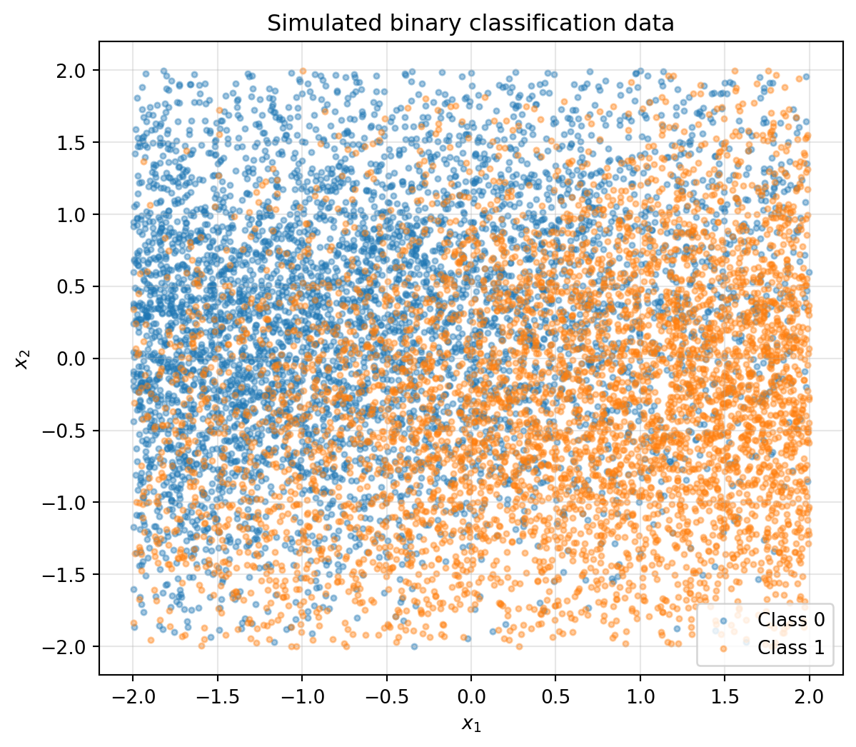
We generate n=10{,}000 observations:
x_1 \sim \mathrm{Uniform}(-2,2)
x_2 is constructed to have correlation \approx 0.5 with x_1, then truncated to [-2,2]
class labels are drawn from
y_i \sim \mathrm{Bernoulli}(p_i),
\qquad
p_i = \sigma(\mathbf x_i^\top \mathbf w_{\text{true}}),
with b=0
The first plot shows the data in feature space.
Even though the relationship is nonlinear in probability space, the classes show structure.
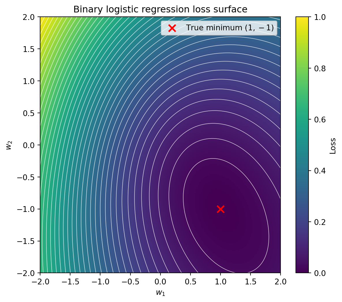
Next, we treat the loss as a function of the parameters:
(w_1, w_2) \mapsto L(w_1, w_2).
We evaluate the binary cross-entropy loss on a grid:
250 values of w_1 between -2 and 2
250 values of w_2 between -2 and 2
Then we plot the contours as a heatmap-style plot. The colors show the actual loss value (normalized for the plot) and the white curves show the contours - each combinarion of w_1 and w_2 on the same contour lines have the same loss value.
You should see:
a smooth convex “bowl”
elliptical contour boundaries that show the curvature of the loss space
and the minimum near the true parameter values (1, -1)
We mark (1,-1) on the plot to emphasize:
The loss surface is minimized at the parameters that generated the data.
Code
def logistic_loss(w, X, y): z = X @ w p =1/ (1+ np.exp(-z)) eps =1e-12# numerical safetyreturn-np.average(y * np.log(p + eps) + (1- y) * np.log(1- p + eps))# Grid for parametersw1_vals = np.linspace(-2, 2, 250)w2_vals = np.linspace(-2, 2, 250)W1, W2 = np.meshgrid(w1_vals, w2_vals)Z = np.zeros_like(W1)for i inrange(W1.shape[0]):for j inrange(W1.shape[1]): w = np.array([W1[i, j], W2[i, j]]) Z[i, j] = logistic_loss(w, X, y)plt.figure(figsize=(7, 6))# Heatmapplt.imshow( Z, extent=[-2, 2, -2, 2], origin="lower", aspect="auto", cmap="viridis")# Contour lines (this is the key R-like part)contour_levels = np.linspace(Z.min(), Z.max(), 40)plt.contour( W1, W2, Z, levels=contour_levels, colors="white", linewidths=0.6, alpha=0.8)# Mark true minimumplt.scatter( w_true[0], w_true[1], color="red", s=80, marker="x", linewidths=2, label="True minimum $(1,-1)$")plt.colorbar(label="Loss")plt.xlabel("$w_1$")plt.ylabel("$w_2$")plt.title("Binary logistic regression loss surface")plt.legend()plt.show()
Step 3: Finding the Minimum
We will treat the loss landscape as a map, and gradient descent as a “hiker” that:
starts at your chosen point (w_1^{(0)}, w_2^{(0)})
and repeatedly optimally moves down the mountain until she reaches a valley
\mathbf w^{(t+1)} = \mathbf w^{(t)} - \eta \nabla L(\mathbf w^{(t)}),
\qquad \eta = 0.01.
In the interactive plot:
Click anywhere on the (w_1,w_2) plane
The algorithm will trace the path to the minimum showing where the optimizer is at each step
Hover over the dots to see what the value is at each iteration
We’ll say a valley has been reached if the norm of the gradient is less than 1 \times 10^{-8} (there’s also a failsafe that stops the routine after 100 iterations)
Code
from bokeh.plotting import figure, showfrom bokeh.models import ColumnDataSource, CustomJS, HoverTool, Divfrom bokeh.layouts import columnfrom bokeh.events import Tapfrom bokeh.io import output_notebookimport matplotlib.pyplot as plt# Enable bokeh in notebookoutput_notebook()# 1. Prepare Data for JS (Downsample for speed)np.random.seed(42)idx_small = np.random.choice(n, 500, replace=False)X_js = X[idx_small].tolist()y_js = y[idx_small].tolist()# 2. Extract Contour Lines from Matplotlibcontour_levels = np.linspace(Z.min(), Z.max(), 25)cs = plt.contour(W1, W2, Z, levels=contour_levels)contour_xs = []contour_ys = []for level_segments in cs.allsegs:for segment in level_segments: contour_xs.append(segment[:, 0].tolist()) contour_ys.append(segment[:, 1].tolist())plt.close() # 3. Setup the Plotp = figure( title="Click to run Gradient Descent", x_range=(-2, 2), y_range=(-2, 2), width=600, height=500, tools="pan,wheel_zoom,reset")# Add the heatmap imagep.image(image=[Z], x=-2, y=-2, dw=4, dh=4, palette="Viridis256")# Add the contour lines (White, semi-transparent)p.multi_line(contour_xs, contour_ys, color="white", alpha=0.4, line_width=1)# (Removed True Min marker as requested)# 4. Setup the Interactive Path# Added 'grad_w1' and 'grad_w2' to the data sourcesource = ColumnDataSource(data=dict(w1=[], w2=[], iter=[], dist=[], grad_w1=[], grad_w2=[]))p.line('w1', 'w2', source=source, line_width=2, color="white", alpha=0.8)points_renderer = p.circle('w1', 'w2', source=source, size=6, color="white", alpha=0.8, hover_color="red")# 5. Add Hover Tool# Added Gradient info to tooltipshover = HoverTool(renderers=[points_renderer], tooltips=[ ("Iteration", "@iter"), ("Dist to Min", "@dist{0.000}"), ("w1", "@w1{0.00}"), ("w2", "@w2{0.00}"), ("Grad w1", "@grad_w1{0.00}"), ("Grad w2", "@grad_w2{0.00}")])p.add_tools(hover)# 6. Summary Divstats_div = Div(text="<b>Click on the plot to start optimization...</b>", width=600, height=30)# 7. The JavaScript Callbackcallback = CustomJS(args=dict(source=source, stats=stats_div, X=X_js, y=y_js, w_true=w_true), code=""" const data = source.data; // Get click coordinates const w1_start = cb_obj.x; const w2_start = cb_obj.y; // Hyperparameters const eta = 0.5; // Increased eta since we are now using mean gradient const max_steps = 100; const tol = 1e-3; // Initialize path arrays const w1_path = []; const w2_path = []; const iter_path = []; const dist_path = []; const grad_w1_path = []; const grad_w2_path = []; let w1 = w1_start; let w2 = w2_start; let final_iter = 0; // Gradient Descent Loop for (let t = 0; t <= max_steps; t++) { final_iter = t; // Compute Gradient first (needed for current step info) let grad_w1 = 0; let grad_w2 = 0; const n = X.length; for (let i = 0; i < n; i++) { const xi = X[i]; const yi = y[i]; const z = xi[0] * w1 + xi[1] * w2; const p = 1 / (1 + Math.exp(-z)); const err = p - yi; grad_w1 += err * xi[0]; grad_w2 += err * xi[1]; } // Average the gradient grad_w1 = grad_w1 / n; grad_w2 = grad_w2 / n; // Record current state w1_path.push(w1); w2_path.push(w2); iter_path.push(t); grad_w1_path.push(grad_w1); grad_w2_path.push(grad_w2); // Calculate Euclidean distance to true min const dist = Math.sqrt(Math.pow(w1 - w_true[0], 2) + Math.pow(w2 - w_true[1], 2)); dist_path.push(dist); // Check stopping condition (Gradient Norm) const grad_norm = Math.sqrt(grad_w1*grad_w1 + grad_w2*grad_w2); if (grad_norm < tol) { break; } // Update weights if not last step if (t < max_steps) { w1 = w1 - eta * grad_w1; w2 = w2 - eta * grad_w2; } } // Update the plot data data['w1'] = w1_path; data['w2'] = w2_path; data['iter'] = iter_path; data['dist'] = dist_path; data['grad_w1'] = grad_w1_path; data['grad_w2'] = grad_w2_path; source.change.emit(); // Update Summary Text const final_w1 = w1_path[w1_path.length-1].toFixed(4); const final_w2 = w2_path[w2_path.length-1].toFixed(4); stats.text = `<b>Result:</b> Stopped at Iteration ${final_iter}. Final w: (${final_w1}, ${final_w2})`;""")p.js_on_event(Tap, callback)# Layout: Plot on top, stats summary belowlayout = column(p, stats_div)show(layout)
Loading BokehJS ...
BokehDeprecationWarning: 'circle() method with size value' was deprecated in Bokeh 3.4.0 and will be removed, use 'scatter(size=...) instead' instead.
This makes two ideas concrete:
Steepest descent means orthogonal to contours
The gradient is perpendicular to level sets of the loss, so the path crosses contours at right angles.
“Locally optimal” does not mean “globally efficient”
Each step is the best immediate decrease, but the full path may curve and zig-zag rather than beelining to the optimum.
Step 4: What you should notice
After clicking a few starting points, you should see consistent patterns:
Regardless of where you start, gradient descent moves toward the same minimum
(this is the convexity advantage of logistic regression).
The path is not straight.
Even though the direction is locally optimal, the global trajectory can be long and winding.
This sets up the core tension of first-order optimization:
Gradient descent is simple and general, but it can be inefficient because it only uses local slope information.
Looking ahead: why step size matters
In this section we fixed \eta = 0.01 and saw the algorithm “work.”
In the next tab, we will focus on the part that makes gradient descent feel hard in practice:
what happens when \eta is too large or too small
why curvature and conditioning matter
and how line search / second-order ideas improve efficiency
Source Code
---title: "06: Gradient Descent"format: html: code-fold: truejupyter: python3---## Why this mattersFor linear regression, we can solve for the optimal parameters in closed form. For logistic regression, **we cannot**.Even though the loss function is convex, there is no equation we can rearrange to obtain$\mathbf w^\*$ directly.Instead, we must *search* for the minimum.This section introduces **gradient descent** as a geometric procedure for navigatinga loss landscape. We will focus on **binary logistic regression with two features** so thatwe can *see* what the algorithm is doing.> This is the last time optimization will look this simple.## The optimization problemRecall the binary logistic regression objective:$$L(\mathbf w)=\frac{1}{n}\sum_{i=1}^n-\big(y_i \log p_i + (1-y_i)\log(1-p_i)\big),\qquadp_i = \sigma(\mathbf x_i^\top \mathbf w).$$From the previous section, we know the gradient:$$\nabla_{\mathbf w} L=\frac{1}{n}\mathbf X^\top(\mathbf p - \mathbf y).$$Written out to show the full mapping of $\mathbf X$ to $\mathbf y$:$$\nabla_{\mathbf w} L=\frac{1}{n}\mathbf X^\top(\sigma(\mathbf X^\top \mathbf w) - \mathbf y).$$where $\sigma(\cdot)$ is the logistic function applied elementwise. Note that $b$ is omitted here as we're assuming that $\mathbf X$ has a column of 1s.We could try to solve for this analytically by finding $\mathbf w^*$ such that:$$\frac{1}{n}\mathbf X^\top(\sigma(\mathbf X^\top \mathbf w^*) - \mathbf y) = \mathbf 0$$Unfortunately, this is not possible due to the pesky logistic function!Instead, we'll need to leverage an **iterative optimization procedure** to find the loss minimizing values of $\mathbf w$.## The gradient descent algorithmGradient descent is a first-order iterative optimization method.Starting from an initial guess $\mathbf w^{(0)}$, we repeatedly apply$$\mathbf w^{(t+1)}=\mathbf w^{(t)}-\eta \nabla_{\mathbf w} L(\mathbf w^{(t)}),$$where:- $\eta > 0$ is the **step size** (learning rate),- $\nabla_{\mathbf w} L$ is evaluated at the *current* parameters.Each update moves the parameters in the direction of steepest descent. In other words, **gradient descent will move from any point to the point $\eta$ away that maximally decreases loss** ### Why the negative gradient?To understand why gradient descent works, let's think about the most efficient move from the current parameter value, $\mathbf w$:$$\underset{\mathbf d}{\max} L(\mathbf w) - L(\mathbf w + \eta\mathbf d)$$where $\eta$ is a very small positive value (almost zero!) and $\mathbf d$ is a **unit vector**. $\mathbf d$ controls the direction of the move of size $\eta$ away from our current point.In words, our goal is to find the **direction** away from the current position that maximizes the decrease in loss.---#### Step 1: Use a first-order approximationBecause $\eta$ is tiny, we can use a first-order Taylor expansion around $\mathbf w$:$$L(\mathbf w + \eta \mathbf d)\approxL(\mathbf w) + \eta \nabla L(\mathbf w)^\top \mathbf d.$$Substitute this into the objective:$$L(\mathbf w) - L(\mathbf w + \eta\mathbf d)\approxL(\mathbf w) - \Big(L(\mathbf w) + \eta \nabla L(\mathbf w)^\top \mathbf d\Big)=-\eta \nabla L(\mathbf w)^\top \mathbf d.$$Drop $\eta$ since it is a constant to get:$$\underset{\mathbf d}{\max}\; -\nabla L(\mathbf w)^\top \mathbf d$$which is equivalent to:$$\underset{\mathbf d}{\min}\; \nabla L(\mathbf w)^\top \mathbf d $$---#### Step 2 (Geometric view): inner product = magnitude × magnitude × cosineNow we can solve this *geometrically* using the fact that an inner product encodes an angle.Let $\mathbf g = \nabla L(\mathbf w)$. Then the objective is $\mathbf g^\top \mathbf d$.By the law of cosines (equivalently, the definition of the dot product), for any two vectors$\mathbf g$ and $\mathbf d$,$$\mathbf g^\top \mathbf d = \|\mathbf g\|_2 \|\mathbf d\|_2 \cos(\theta),$$where $\theta$ is the angle between $\mathbf g$ and $\mathbf d$.But we are restricting to unit vectors $\mathbf d$, so $\|\mathbf d\|_2 = 1$. Therefore:$$\mathbf g^\top \mathbf d = \|\mathbf g\|_2 \cos(\theta).$$The only quantity we can control is the angle $\theta$.---#### Step 3: maximize cosine by aligning directionsBecause$$-1 \le \cos(\theta) \le 1,$$the minimum value occurs when $\cos(\theta) = -1$, i.e. when the direction moves **exactly opposite the gradient**.That happens exactly when $\mathbf d$ points in the *opposite direction* as $\mathbf g$:$$\mathbf d^* = \frac{-\mathbf g}{\|\mathbf g\|_2}= \frac{-\nabla L(\mathbf w)}{\|\nabla L(\mathbf w)\|_2}.$$---## Iterative Gradient Descent and Covergence GuaranteesUsing this identity, an iterative strategy for finding a **local** minimum for any loss function for which we can evaluate the value of the gradient at any point arises:1. Choose a starting point, $\mathbf w^{(0)}$, and a small **step-size**, $\eta$. Set $t = 0$.2. Evaluate the gradient for the unknowns with respect to the loss at $t$: $\nabla L(\mathbf w^{(t)})$3. Set $\mathbf w^{(t+1)} = \mathbf w^{(t)} - \eta \nabla L(\mathbf w^{(t)})$4. Repeat steps 2 and 3 until convergence.This approach is **guaranteed** to find a local minimum *eventually* since each step is guaranteed to find a $\mathbf w^{(t + 1)}$ that has weakly lower loss than the previous $\mathbf w$. If we are at a critical point (e.g. $\nabla L(\mathbf w^{(t)}) = \mathbf 0$), note that the update step goes to zero and we no longer move!In practice, we can only guarantee convergence has occurred if the following to conditions are met:1. $t = \infty$2. $\eta = \epsilon$ where $\epsilon$ is the smallest positive number greater than 0Unfortunately, neither of these conditions are practically achievable. Instead, we typically say that it's "good enough" and ready to stop if one (or more) of the following conditions is met:1. **Gradient norm** $$ \|\nabla_{\mathbf w} L\| < \varepsilon $$2. **Relative loss change** $$ \frac{|L^{(t)} - L^{(t-1)}|}{L^{(t-1)}} < \text{tol} $$3. **Maximum iterations** (a safety bound)All three reflect the same idea: we stop when further progress is negligible.## Gradient descent in action (binary logistic regression with two features)Now we will *watch* gradient descent work in the simplest setting where we can actually see the loss landscape.We will use:- **two classes** ($y \in \{0,1\}$),- **two features** ($\mathbf x_i \in \mathbb R^2$),- **no intercept** ($b=0$, so you can think of $\mathbf X$ as already containing a column of ones if you want an intercept later),- and a ground-truth parameter vector $$ \mathbf w_{\text{true}} = \begin{bmatrix} 1 \\ -1 \end{bmatrix}. $$This gives us a clean “sandbox” where:1. We can visualize the data in $(x_1, x_2)$ space.2. We can visualize the loss surface in $(w_1, w_2)$ space.3. We can click anywhere in parameter space and *see* gradient descent walk to the minimum.> This is the last time optimization will feel like geometry on a 2D picture.> The goal is to build intuition here before we lose the ability to “see” the landscape.---### Step 1: Simulate a dataset we can visualizeWe generate $n=10{,}000$ observations:- $x_1 \sim \mathrm{Uniform}(-2,2)$- $x_2$ is constructed to have correlation $\approx 0.5$ with $x_1$, then truncated to $[-2,2]$- class labels are drawn from $$ y_i \sim \mathrm{Bernoulli}(p_i), \qquad p_i = \sigma(\mathbf x_i^\top \mathbf w_{\text{true}}), $$ with $b=0$The first plot shows the data in feature space. Even though the relationship is nonlinear in probability space, the classes show structure.```{python}import numpy as npimport matplotlib.pyplot as pltfrom scipy.stats import truncnorm# -----------------------------# Data generation# -----------------------------np.random.seed(42)n =10_000# x1 ~ Uniform(-2, 2)x1 = np.random.uniform(-2, 2, n)# x2 correlated with x1 (~0.5)eps = np.random.normal(0, 1, n)x2_raw =0.5* x1 + np.sqrt(1-0.5**2) * eps# Truncate x2 to [-2, 2]a, b = (-2- np.mean(x2_raw)) / np.std(x2_raw), (2- np.mean(x2_raw)) / np.std(x2_raw)x2 = truncnorm.rvs(a, b, loc=np.mean(x2_raw), scale=np.std(x2_raw), size=n)X = np.column_stack([x1, x2])# True parametersw_true = np.array([1.0, -1.0])# Generate labelslogits = X @ w_truep =1/ (1+ np.exp(-logits))y = np.random.binomial(1, p)# -----------------------------# Plot: feature space# -----------------------------plt.figure(figsize=(7, 6))plt.scatter(x1[y ==0], x2[y ==0], s=8, alpha=0.4, label="Class 0")plt.scatter(x1[y ==1], x2[y ==1], s=8, alpha=0.4, label="Class 1")plt.xlabel("$x_1$")plt.ylabel("$x_2$")plt.title("Simulated binary classification data")plt.legend()plt.grid(alpha=0.3)plt.show()```---### Step 2: The Loss LandscapeNext, we treat the **loss** as a function of the parameters:$$(w_1, w_2) \mapsto L(w_1, w_2).$$We evaluate the binary cross-entropy loss on a grid:- $250$ values of $w_1$ between $-2$ and $2$- $250$ values of $w_2$ between $-2$ and $2$Then we plot the contours as a heatmap-style plot. The colors show the actual loss value (normalized for the plot) and the white curves show the **contours** - each combinarion of $w_1$ and $w_2$ on the same contour lines have the same loss value. You should see:- a smooth convex “bowl”- elliptical contour boundaries that show the ***curvature*** of the loss space- and the minimum near the true parameter values $(1, -1)$We mark $(1,-1)$ on the plot to emphasize:> The loss surface is minimized at the parameters that generated the data.```{python}def logistic_loss(w, X, y): z = X @ w p =1/ (1+ np.exp(-z)) eps =1e-12# numerical safetyreturn-np.average(y * np.log(p + eps) + (1- y) * np.log(1- p + eps))# Grid for parametersw1_vals = np.linspace(-2, 2, 250)w2_vals = np.linspace(-2, 2, 250)W1, W2 = np.meshgrid(w1_vals, w2_vals)Z = np.zeros_like(W1)for i inrange(W1.shape[0]):for j inrange(W1.shape[1]): w = np.array([W1[i, j], W2[i, j]]) Z[i, j] = logistic_loss(w, X, y)plt.figure(figsize=(7, 6))# Heatmapplt.imshow( Z, extent=[-2, 2, -2, 2], origin="lower", aspect="auto", cmap="viridis")# Contour lines (this is the key R-like part)contour_levels = np.linspace(Z.min(), Z.max(), 40)plt.contour( W1, W2, Z, levels=contour_levels, colors="white", linewidths=0.6, alpha=0.8)# Mark true minimumplt.scatter( w_true[0], w_true[1], color="red", s=80, marker="x", linewidths=2, label="True minimum $(1,-1)$")plt.colorbar(label="Loss")plt.xlabel("$w_1$")plt.ylabel("$w_2$")plt.title("Binary logistic regression loss surface")plt.legend()plt.show()```---### Step 3: Finding the MinimumWe will treat the loss landscape as a map, and gradient descent as a “hiker” that:- starts at your chosen point $(w_1^{(0)}, w_2^{(0)})$- and repeatedly optimally moves down the mountain until she reaches a valley $$ \mathbf w^{(t+1)} = \mathbf w^{(t)} - \eta \nabla L(\mathbf w^{(t)}), \qquad \eta = 0.01. $$In the interactive plot:- Click anywhere on the $(w_1,w_2)$ plane- The algorithm will trace the path to the minimum showing where the optimizer is at each step- Hover over the dots to see what the value is at each iteration- We'll say a valley has been reached if the norm of the gradient is less than $1 \times 10^{-8}$ (there's also a failsafe that stops the routine after 100 iterations)```{python}from bokeh.plotting import figure, showfrom bokeh.models import ColumnDataSource, CustomJS, HoverTool, Divfrom bokeh.layouts import columnfrom bokeh.events import Tapfrom bokeh.io import output_notebookimport matplotlib.pyplot as plt# Enable bokeh in notebookoutput_notebook()# 1. Prepare Data for JS (Downsample for speed)np.random.seed(42)idx_small = np.random.choice(n, 500, replace=False)X_js = X[idx_small].tolist()y_js = y[idx_small].tolist()# 2. Extract Contour Lines from Matplotlibcontour_levels = np.linspace(Z.min(), Z.max(), 25)cs = plt.contour(W1, W2, Z, levels=contour_levels)contour_xs = []contour_ys = []for level_segments in cs.allsegs:for segment in level_segments: contour_xs.append(segment[:, 0].tolist()) contour_ys.append(segment[:, 1].tolist())plt.close() # 3. Setup the Plotp = figure( title="Click to run Gradient Descent", x_range=(-2, 2), y_range=(-2, 2), width=600, height=500, tools="pan,wheel_zoom,reset")# Add the heatmap imagep.image(image=[Z], x=-2, y=-2, dw=4, dh=4, palette="Viridis256")# Add the contour lines (White, semi-transparent)p.multi_line(contour_xs, contour_ys, color="white", alpha=0.4, line_width=1)# (Removed True Min marker as requested)# 4. Setup the Interactive Path# Added 'grad_w1' and 'grad_w2' to the data sourcesource = ColumnDataSource(data=dict(w1=[], w2=[], iter=[], dist=[], grad_w1=[], grad_w2=[]))p.line('w1', 'w2', source=source, line_width=2, color="white", alpha=0.8)points_renderer = p.circle('w1', 'w2', source=source, size=6, color="white", alpha=0.8, hover_color="red")# 5. Add Hover Tool# Added Gradient info to tooltipshover = HoverTool(renderers=[points_renderer], tooltips=[ ("Iteration", "@iter"), ("Dist to Min", "@dist{0.000}"), ("w1", "@w1{0.00}"), ("w2", "@w2{0.00}"), ("Grad w1", "@grad_w1{0.00}"), ("Grad w2", "@grad_w2{0.00}")])p.add_tools(hover)# 6. Summary Divstats_div = Div(text="<b>Click on the plot to start optimization...</b>", width=600, height=30)# 7. The JavaScript Callbackcallback = CustomJS(args=dict(source=source, stats=stats_div, X=X_js, y=y_js, w_true=w_true), code=""" const data = source.data; // Get click coordinates const w1_start = cb_obj.x; const w2_start = cb_obj.y; // Hyperparameters const eta = 0.5; // Increased eta since we are now using mean gradient const max_steps = 100; const tol = 1e-3; // Initialize path arrays const w1_path = []; const w2_path = []; const iter_path = []; const dist_path = []; const grad_w1_path = []; const grad_w2_path = []; let w1 = w1_start; let w2 = w2_start; let final_iter = 0; // Gradient Descent Loop for (let t = 0; t <= max_steps; t++) { final_iter = t; // Compute Gradient first (needed for current step info) let grad_w1 = 0; let grad_w2 = 0; const n = X.length; for (let i = 0; i < n; i++) { const xi = X[i]; const yi = y[i]; const z = xi[0] * w1 + xi[1] * w2; const p = 1 / (1 + Math.exp(-z)); const err = p - yi; grad_w1 += err * xi[0]; grad_w2 += err * xi[1]; } // Average the gradient grad_w1 = grad_w1 / n; grad_w2 = grad_w2 / n; // Record current state w1_path.push(w1); w2_path.push(w2); iter_path.push(t); grad_w1_path.push(grad_w1); grad_w2_path.push(grad_w2); // Calculate Euclidean distance to true min const dist = Math.sqrt(Math.pow(w1 - w_true[0], 2) + Math.pow(w2 - w_true[1], 2)); dist_path.push(dist); // Check stopping condition (Gradient Norm) const grad_norm = Math.sqrt(grad_w1*grad_w1 + grad_w2*grad_w2); if (grad_norm < tol) { break; } // Update weights if not last step if (t < max_steps) { w1 = w1 - eta * grad_w1; w2 = w2 - eta * grad_w2; } } // Update the plot data data['w1'] = w1_path; data['w2'] = w2_path; data['iter'] = iter_path; data['dist'] = dist_path; data['grad_w1'] = grad_w1_path; data['grad_w2'] = grad_w2_path; source.change.emit(); // Update Summary Text const final_w1 = w1_path[w1_path.length-1].toFixed(4); const final_w2 = w2_path[w2_path.length-1].toFixed(4); stats.text = `<b>Result:</b> Stopped at Iteration ${final_iter}. Final w: (${final_w1}, ${final_w2})`;""")p.js_on_event(Tap, callback)# Layout: Plot on top, stats summary belowlayout = column(p, stats_div)show(layout)```This makes two ideas concrete:1. **Steepest descent means orthogonal to contours** The gradient is perpendicular to level sets of the loss, so the path crosses contours at right angles.2. **“Locally optimal” does not mean “globally efficient”** Each step is the best immediate decrease, but the full path may curve and zig-zag rather than beelining to the optimum.---### Step 4: What you should noticeAfter clicking a few starting points, you should see consistent patterns:- **Regardless of where you start**, gradient descent moves toward the same minimum (this is the convexity advantage of logistic regression).- **The path is not straight.** Even though the direction is locally optimal, the global trajectory can be long and winding.This sets up the core tension of first-order optimization:> Gradient descent is simple and general, but it can be inefficient because it only uses local slope information.---### Looking ahead: why step size mattersIn this section we fixed $\eta = 0.01$ and saw the algorithm “work.”In the next tab, we will focus on the part that makes gradient descent *feel hard in practice*:- what happens when $\eta$ is too large or too small- why curvature and conditioning matter- and how line search / second-order ideas improve efficiency